What is the standard error?
Standard error statistics are a class of statistics that are provided as output in many inferential statistics, but function as descriptive statistics. Specifically, the term standard error refers to a group of statistics that provide information about the dispersion of the values within a set. Use of the standard error statistic presupposes the user is familiar with the central limit theorem and the assumptions of the data set with which the researcher is working.
The central limit theorem is a foundation assumption of all parametric inferential statistics. Its application requires that the sample is a random sample, and that the observations on each subject are independent of the observations on any other subject. It states that regardless of the shape of the parent population, the sampling distribution of means derived from a large number of random samples drawn from that parent population will exhibit a normal distribution (1). Specifically, although a small number of samples may produce a non-normal distribution, as the number of samples increases (that is, as n increases), the shape of the distribution of sample means will rapidly approach the shape of the normal distribution. A second generalization from the central limit theorem is that as n increases, the variability of sample means decreases (2). This is important because the concept of sampling distributions forms the theoretical foundation for the mathematics that allows researchers to draw inferences about populations from samples.
Researchers typically draw only one sample. It is not possible for them to take measurements on the entire population. They have neither the time nor the money. For the same reasons, researchers cannot draw many samples from the population of interest. Therefore, it is essential for them to be able to determine the probability that their sample measures are a reliable representation of the full population, so that they can make predictions about the population. The determination of the representativeness of a particular sample is based on the theoretical sampling distribution the behavior of which is described by the central limit theorem. The standard error statistics are estimates of the interval in which the population parameters may be found, and represent the degree of precision with which the sample statistic represents the population parameter. The smaller the standard error, the closer the sample statistic is to the population parameter. The standard error of a statistic is therefore the standard deviation of the sampling distribution for that statistic (3)
How, one might ask, does the standard error differ from the standard deviation? The two concepts would appear to be very similar. They are quite similar, but are used differently. The standard deviation is a measure of the variability of the sample. The standard error is a measure of the variability of the sampling distribution. Just as the standard deviation is a measure of the dispersion of values in the sample, the standard error is a measure of the dispersion of values in the sampling distribution. That is, of the dispersion of means of samples if a large number of different samples had been drawn from the population.
Standard error of the mean
The standard error of a sample mean is represented by the following formula:
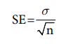
That is, the standard error is equal to the standard deviation divided by the square root of the sample size, n. This shows that the larger the sample size, the smaller the standard error. (Given that the larger the divisor, the smaller the result and the smaller the divisor, the larger the result.) The symbol for standard error of the mean is sM or when symbols are difficult to produce, it may be represented as, S.E. mean, or more simply as SEM.
The standard error of the mean can provide a rough estimate of the interval in which the population mean is likely to fall. The SEM, like the standard deviation, is multiplied by 1.96 to obtain an estimate of where 95% of the population sample means are expected to fall in the theoretical sampling distribution. To obtain the 95% confidence interval, multiply the SEM by 1.96 and add the result to the sample mean to obtain the upper limit of the interval in which the population parameter will fall. Then subtract the result from the sample mean to obtain the lower limit of the interval. The resulting interval will provide an estimate of the range of values within which the population mean is likely to fall. In fact, the level of probability selected for the study (typically P < 0.05) is an estimate of the probability of the mean falling within that interval. This interval is a crude estimate of the confidence interval within which the population mean is likely to fall. A more precise confidence interval should be calculated by means of percentiles derived from the t-distribution.
Another use of the value, 1.96 ± SEM is to determine whether the population parameter is zero. If the interval calculated above includes the value, “0”, then it is likely that the population mean is zero or near zero. Consider, for example, a researcher studying bedsores in a population of patients who have had open heart surgery that lasted more than 4 hours. Suppose the mean number of bedsores was 0.02 in a sample of 500 subjects, meaning 10 subjects developed bedsores. If the standard error of the mean is 0.011, then the population mean number of bedsores will fall approximately between 0.04 and -0.0016. This is interpreted as follows: The population mean is somewhere between zero bedsores and 20 bedsores. Given that the population mean may be zero, the researcher might conclude that the 10 patients who developed bedsores are outliers. That in turn should lead the researcher to question whether the bedsores were developed as a function of some other condition rather than as a function of having heart surgery that lasted longer than 4 hours.
Standard error of the estimate
The standard error of the estimate (S.E.est) is a measure of the variability of predictions in a regression. Specifically, it is calculated using the following formula:
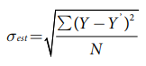
Where Y is a score in the sample and Y’ is a predicted score.
Therefore, the standard error of the estimate is a measure of the dispersion (or variability) in the predicted scores in a regression. In a scatterplot in which the S.E.est is small, one would therefore expect to see that most of the observed values cluster fairly closely to the regression line. When the S.E.est is large, one would expect to see many of the observed values far away from the regression line as in Figures 1 and 2.
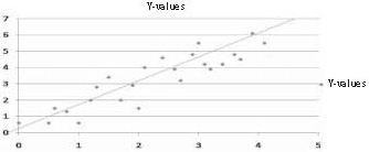
Figure 1. Low S.E. estimate – Predicted Y values close to regression line
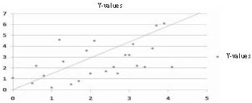
Figure 2. Large S.E. estimate – Predicted Y values scattered widely above and below regression line
Other standard errors
Every inferential statistic has an associated standard error. Although not always reported, the standard error is an important statistic because it provides information on the accuracy of the statistic (4). As discussed previously, the larger the standard error, the wider the confidence interval about the statistic. In fact, the confidence interval can be so large that it is as large as the full range of values, or even larger. In that case, the statistic provides no information about the location of the population parameter. And that means that the statistic has little accuracy because it is not a good estimate of the population parameter.
In this way, the standard error of a statistic is related to the significance level of the finding. When the standard error is large relative to the statistic, the statistic will typically be non-significant. However, if the sample size is very large, for example, sample sizes greater than 1,000, then virtually any statistical result calculated on that sample will be statistically significant. For example, a correlation of 0.01 will be statistically significant for any sample size greater than 1500. However, a correlation that small is not clinically or scientifically significant. When effect sizes (measured as correlation statistics) are relatively small but statistically significant, the standard error is a valuable tool for determining whether that significance is due to good prediction, or is merely a result of power so large that any statistic is going to be significant. The answer to the question about the importance of the result is found by using the standard error to calculate the confidence interval about the statistic. When the finding is statistically significant but the standard error produces a confidence interval so wide as to include over 50% of the range of the values in the dataset, then the researcher should conclude that the finding is clinically insignificant (or unimportant). This is true because the range of values within which the population parameter falls is so large that the researcher has little more idea about where the population parameter actually falls than he or she had before conducting the research.
When the statistic calculated involves two or more variables (such as regression, the t-test) there is another statistic that may be used to determine the importance of the finding. That statistic is the effect size of the association tested by the statistic. Consider, for example, a regression. Suppose the sample size is 1,500 and the significance of the regression is 0.001. The obtained P-level is very significant. However, one is left with the question of how accurate are predictions based on the regression? The effect size provides the answer to that question. In a regression, the effect size statistic is the Pearson Product Moment Correlation Coefficient (which is the full and correct name for the Pearson r correlation, often noted simply as, R). If the Pearson R value is below 0.30, then the relationship is weak no matter how significant the result. An R of 0.30 means that the independent variable accounts for only 9% of the variance in the dependent variable. The 9% value is the statistic called the coefficient of determination. It is calculated by squaring the Pearson R. It is an even more valuable statistic than the Pearson because it is a measure of the overlap, or association between the independent and dependent variables. (See Figure 3).
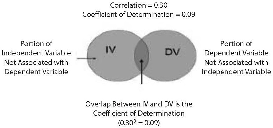
Figure 3. Coefficient of determination
The great value of the coefficient of determination is that through use of the Pearson R statistic and the standard error of the estimate, the researcher can construct a precise estimate of the interval in which the true population correlation will fall. This capability holds true for all parametric correlation statistics and their associated standard error statistics. In fact, even with non-parametric correlation coefficients (i.e., effect size statistics), a rough estimate of the interval in which the population effect size will fall can be estimated through the same type of calculations.
However, many statistical results obtained from a computer statistical package (such as SAS, STATA, or SPSS) do not automatically provide an effect size statistic. In most cases, the effect size statistic can be obtained through an additional command. For example, the effect size statistic for ANOVA is the Eta-square. The SPSS ANOVA command does not automatically provide a report of the Eta-square statistic, but the researcher can obtain the Eta-square as an optional test on the ANOVA menu. For some statistics, however, the associated effect size statistic is not available. When an effect size statistic is not available, the standard error statistic for the statistical test being run is a useful alternative to determining how accurate the statistic is, and therefore how precise is the prediction of the dependent variable from the independent variable.
Summary and conclusions
The standard error is a measure of dispersion similar to the standard deviation. However, while the standard deviation provides information on the dispersion of sample values, the standard error provides information on the dispersion of values in the sampling distribution associated with the population of interest from which the sample was drawn. Standard error statistics measure how accurate and precise the sample is as an estimate of the population parameter. It is particularly important to use the standard error to estimate an interval about the population parameter when an effect size statistic is not available.
The standard error is not the only measure of dispersion and accuracy of the sample statistic. It is, however, an important indicator of how reliable an estimate of the population parameter the sample statistic is. Taken together with such measures as effect size, p-value and sample size, the effect size can be a very useful tool to the researcher who seeks to understand the reliability and accuracy of statistics calculated on random samples.