Introduction
Power is a critically important concept for researchers because it is the hub around which the achievement of statistical significance revolves. Statistical significance is the research factor that researchers use to determine if an intervention changes an outcome. That determination cannot be achieved with insufficient power. On the other hand, extremely high power might influence a researcher to give more weight to a statistical result than the clinical situation warrants. The purpose of this paper is to review the foundations of statistical power, and to provide information on how it is used to increase the probability of obtaining reliable information from research studies.
Meaning of power
In the context of research, power refers to the likelihood that a researcher will find a significant result (an effect) in a sample if such an effect exists in the population being studied(1). The way a researcher poses the question about a significant result is through use of the null hypothesis. The null hypothesis always proposes the hypothesis that there is no difference between the experimental and control groups for the variable being tested. The null hypothesis is what all inferential statistics test.
The values that Power can take range from 0.0 to 1.0. These values cannot be interpreted directly. However, the probability of a Type II error is calculated as 1-Power. Therefore, the higher the power, the more likely one is to detect a significant effect. When power is low, it is unlikely that the researcher will find an effect, and thus reject the null hypothesis, even when there is a real difference between the experimental and control groups. The effect the researcher is trying to find is the alternate hypothesis – which is, of course, the study hypothesis. That is typically worded in a fashion similar to this statement: “There is a difference between the experimental and control groups”. Described in a different way, power is the likelihood that a false null hypothesis (that is, there is an effect in the full population), will be rejected (see Table 1). When a null hypothesis is rejected, the alternate hypothesis is accepted. Indirectly, this means that power is a key factor in the researcher being able to draw correct conclusions from sample data.
Table 1. Type I and type II errors
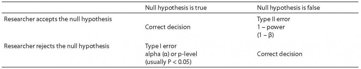
Problems with power can lead to a variety of errors in interpretation of statistical results. They might lead the researcher to conclude there is no effect from an experimental treatment when in fact an effect does exist in the population. They might lead the researcher to incorrectly conclude that there is an important effect when the fact is that there is an effect, but it is so small as to be inconsequential. Therefore, it is important for every researcher to understand the meaning of power and the factors that affect statistical power so that statistical conclusions are more accurate and reliable.
Foundations of statistical power
Statistical power is primarily a function of three factors (see Figure 1), and secondarily of one additional factor. The primary factors are sample size, effect size and level of significance used in the study.
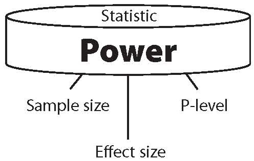
Figure 1. The three components of power.
The secondary factor is the power of the statistic used. When any two of the primary factors are known, the third can be calculated from the other two. And when all three factors are known, the power of a statistical result can be calculated. Equally important, when power and just one of the primary factors – effect size – are known, the sample size needed to achieve statistical significance can be calculated.
Sample size
The first factor – and the factor most directly under the control of the researcher – is sample size. In fact, sample size is often the only factor that the researcher can realistically control. Sample size has a very direct and very strong effect on statistical power in any study. Simply put, the larger the sample, the greater the statistical power. Conversely, when sample size is small, power is weak. This is logically true because we know that if the researcher could measure an entire, large population, then the researcher would have complete power to find any effects that might exist in the population for the variables measured. In fact, inferential statistics would be unnecessary. Inferential statistics allow the researcher to infer (estimate) the effect size in the population from a sample. If the entire population were measured, there would be no need to estimate the effect because the effect size would be directly known. In other words, if a researcher measures the entire population, the power is 100% because any effect will be detected. Furthermore, if the researcher measures the entire population, there is no danger of the sample being a poor estimate of the population. Although sampling is not the topic of this paper, it is necessary to note that inferential statistics are only as accurate as the sample is representative of the population. Therefore, none of the theories that support sample research apply if the researcher obtains a biased sample (that is, a sample that is not representative of the population). With a study that uses the entire population, there is no danger of an unrepresentative result.
Conversely, it is well known that very small sample sizes are unreliable estimators of a population parameter. No sensible researcher would try to predict the effect of a new drug on a population of millions by sampling one individual. The high likelihood of an erroneous conclusion with an “N of one” is so well known as to constitute a cliché. A sample size of 5 individuals would be almost as bad for testing the effects of a new drug. That sample size is too small to fully represent a large population. In fact, a heuristic often used in research is that samples of less than 30 are considered small sample sizes and should be used only for pilot studies.
The question then arises, “What sample size does a researcher need to detect an effect if it exists in the population?” The typical way to find the answer to that question is called “power analysis” and it involves performing mathematical calculations to determine what sample size is needed to detect an effect of a certain size. In order to calculate the sample size needed, the researcher needs to know the effect size. It must also be noted that sometimes a researcher discovers that a moderate effect size is not found to be statistically significant. A power analysis might be performed in this case to discover if the problem with statistical significance was insufficient power due to an inadequate sample size.
There are a variety of programs available via the Internet to assist the researcher to quickly determine sample size. One of the most useful can be found on the University of Iowa web site (2): http://www.stat.uiowa.edu/črlenth/Power/index.html. The user identifies the statistic to be used, and inputs information about effect size and the program will calculate the sample size required for a particular power level. For example, suppose the researcher plans to run a study on two randomly assigned samples, one of which has received an experimental treatment and the other has not. The typical test used to test group differences is the t-test. The home screen offers a screen menu on the site with a variety of statistical tests. When the user double clicks on one of the statistics in that menu, the graphical user interface (GUI) calculator comes up on the screen (Figure 2).
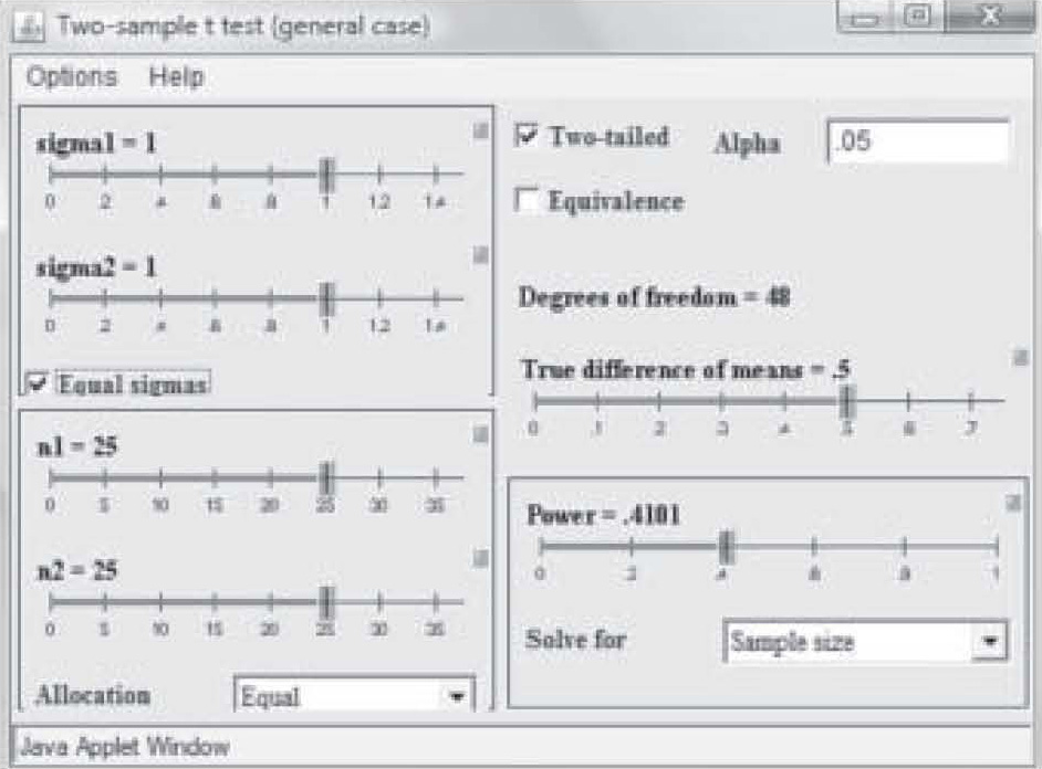
Figure 2. University of Iowa online power calculator – test calculator.
Note on Figure 2 that effect size is 0.50 but power is only 0.41. Those levels result in a needed sample size of only 25 in each study group (total N = 50). However, that power is too weak to use in a research study, so in Figure 3, the power has been reset to 0.80 by simply clicking and dragging on the bar in the Power box. Notice that the per-group sample size required to find an effect size of 0.50 at 0.80 power has increased to N = 63. Now suppose the researcher wants a power of 0.80 but suspects the effect size will be only 0.35. Figure 4 shows the sample size required to find that effect has raised to 129 per group. In this way, the researcher can use the
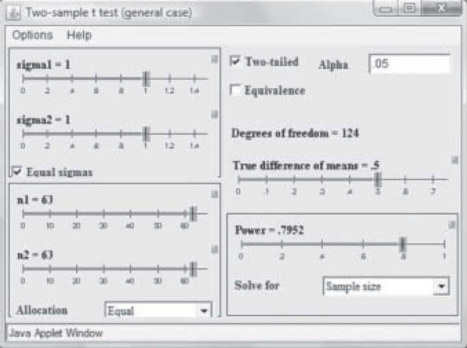
Figure 3. Sample size needed with power changed to 0.80.
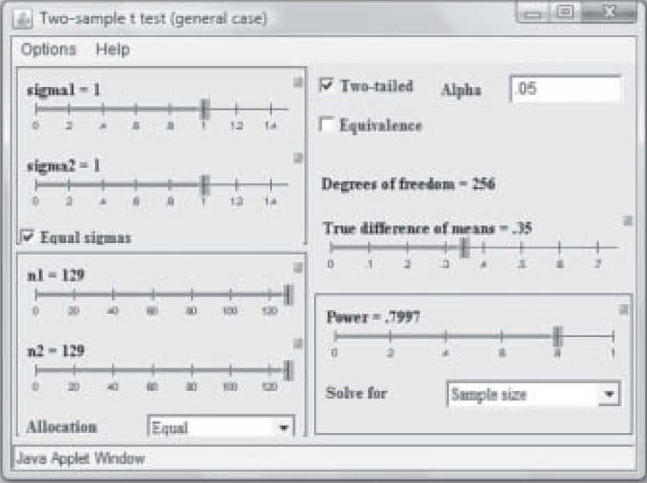
Figure 4. Sample size change due to change in effect size.
University of Iowa site to determine the sample size needed to achieve significance for a particular effect size and power level. The reader should note that there is a set of directions for using the University of Iowa power calculator at the following web site:http://hschealth.uchsc.edu/son/pdf3/PowerCalculatorsHowTo.pdf. Another site with additional power and sample size calculations can be found at Harvard University’s site: http://hedwig.mgh.harvard.edu/sample_size/size.html
Effect size
Effect size represents the size of the difference between the treated and untreated groups in a research study, that is, it represents the magnitude of the treatment effect (3). It is to test for effect size that researchers perform experimental studies. That is, researchers typically seek to discover if a treatment produces an effect in the experimental subjects, and if so, what size of an effect did the treatment produce? People often think of correlation when they think of effect size. This is natural because correlations are measures of effect size. However, difference statistics such as the t-test and ANOVA also have an effect size. In fact, the effect size measure for the t-test is the point biserial correlation coefficient, and the eta-squared statistic is the effect size measure for ANOVA.
All statistics used to measure treatment effects – that is, all inferential statistics – have an associated effect size measure. No researcher should ever report significance without also reporting the effect size. While the statistically sophisticated reader can estimate effect size from the sample size and significance level, there should never be the need for a reader to perform that calculation. It is the responsibility of the researcher to provide the reader with the information the reader needs to properly evaluate the study.
As mentioned earlier, a significance level and sample size report can result in a misled reader. This is because a very large sample size, that is, 1,000 or more subjects, will produce significant results even for very small effect sizes. Suppose, for example, the researcher reports a significant correlation between the use of some herb and a shorter course of a common illness, such as common cold. Readers might assume from the significant result that if they only take the herb when they come down with a cold, they will get well much faster. However, if the sample size was 2,500 and the duration of the cold in the herb group only 5 minutes shorter, that result would be statistically significant. It would not be clinically significant. It is important for the researcher to understand that extremely high power levels will produce statistically significant results, even for minuscule effect sizes.
There is an important difference between statistical significance and clinical significance. It can be difficult for the average member of the public to understand that kind of a difference. However, researchers should be cognizant of the fact that while large sample sizes are very good for producing reliable results, they also produce significant results for almost every effect size. When drugs, herbal remedies, and other chemically active agents are the subject of research studies, it is important to consider not only statistical significance. Effect size must be considered as well. Very small effect sizes (effect sizes of 0.30 or less) should be viewed with skepticism. They may be random rather than reliable effects in a large population. And they mean that the treatment produced a small effect on the dependent variable. The effect size should be squared to evaluate the percentage of variance in the dependent variable produced by the independent variable. Thus, an effect size of 0.30 means that the treatment accounted for only 9% of the difference in the dependent variable. Ninety-one percent of the effect on the dependent variable was not accounted for by the independent variable. Therefore, the treatment effect was too small to recommend that people spend money on the treatment – especially since the treatment (drug or herb remedy) will almost certainly have deleterious side effects in some people. The risk of side effects is not worth the small potential benefit.
Given that the researcher may not know what effect size to expect from a treatment, how then shall the calculators be used to determine sample size needed? There are two ways that the researcher may select an effect size: prior studies and minimal effect size of interest.
If prior studies have been performed, the effect size reported may be the researcher’s best estimate of the effect size likely to be caused by the treatment. When such studies are available, prior reports of the effect size should be considered. However, the more common situation for original research is that either there are no prior studies of the treatment effect, or the prior studies were too dissimilar to the proposed study. Or perhaps prior studies were performed in an animal species different from that the proposed study intends to use.
The minimal effect size has no accepted standard. It may differ among situations. For example, if there is a serious disease with no effective treatment, the minimal effect size may be relatively small. If the new drug accounts for only 10% of the improvement in outcomes, that may be worthwhile to patients. To achieve that 10%, the effect size must be 0.32 and this means that 32% of the change in the dependent variable can be attributed to the treatment. However, if there is an accepted treatment with a known effect, the minimum effect size should, in most cases, be an effect greater than the effect of the known treatment. For example, if the known treatment exhibits an effect size of 0.45, the new drug should have an effect of at least 0.55. Or perhaps its effect size is only 0.45 but the new drug produces substantially fewer (or less severe) side effects. As can be seen, the selection of a minimum effect size is a product of the researcher’s knowledge of related research and good judgment.
In human clinical research, the researcher determines the smallest effect size that would be clinically important. If the results are statistically significant due to a large sample size, but the clinical effect in the human population is negligible, then the results are not clinically significant. This is a different standard than for statistical significance.
As an example, consider that a medical researcher is studying sepsis caused by non-MRSA Staphylococcus aureus. The standard drug used produces a survival rate of 60%. A new drug produces a survival rate of 62% and in a sample of 2,204 subjects the effect sizes are 0.77 and 0.79 respectively (rounded). Generally, the new drug will be much more expensive. Is a 2% change in the outcome worth millions of dollars a year more in treatment costs? If the treatment costs are the same, are the side effects different? What effect size would the researcher demand in this type of drug study if either the cost of the new drug were much higher or if it produced unpleasant or dangerous side effects? These are the kinds of questions that must be considered when the researcher selects a minimum effect size.
Once the requisite effect size has been determined, the researcher simply sets the effect size in the calculator to that minimal effect size and the calculator determines the sample size needed to detect that effect size. If an effect exists but the effect is less than the minimal effect size of interest, it will not achieve significance. If there is an effect at or larger than the minimal effect size of interest, the result will be significant. In this way, the researcher is able to plan a pilot study that will not only assist with pretesting instruments and data collection procedures, but will also improve the likelihood that the full study will be worth performing.
Significance level
The significance level, also called the P-level, of a study is typically set by scientific convention. For example, in most social science studies the significance level should be 0.05 or less. In some drug studies, the P-level must be much lower than 0.05 because of governmental review requirements for effectiveness and safety. Significance represents the likelihood of a Type I error. That is, it is the likelihood that the researcher will falsely claim a significant effect has been found when there is no effect in the population (see Table 1).
With a very small sample size or a sample that poorly represents the population, there is always a high probability that no effect will be found, or conversely, that any effect found in the sample will not exist in the full population. Therefore, when performing pilot studies with small sample sizes, it is common for a researcher to set the significance level higher that usual in order to compensate for the small sample size. Thus, when the conventional significance level is P < 0.05, a pilot study might use a P-level of 0.10 or even 0.20. The purpose of the higher significance level in a pilot study is to avoid abandoning what might otherwise be a promising line of research on the basis of a pilot study that finds no effect for the treatment. Given the current tendency of editors to publish reports of pilot studies, readers should always keep in mind that studies reporting an effect at the P < 0.10 or higher levels should not be applied to patient populations, or should be applied to human populations only with the utmost oversight and care. Such studies are likely to result in population effects very different from the effects seen in the study sample.
It should also be noted that when the researcher publishes a report of a pilot study using an inflated alpha level, the sample size may be quite a bit smaller to obtain significance at the same power level and effect size. Note in Figure 5 that at a power of 0.80 and an effect size of 0.35, a sample of only 74 in each group was needed to obtain “significance” when the P-level was set to 0.20. With a p-level of 0.05, the same study requires a sample size of 129 in each group to achieve significance (see Figure 4).
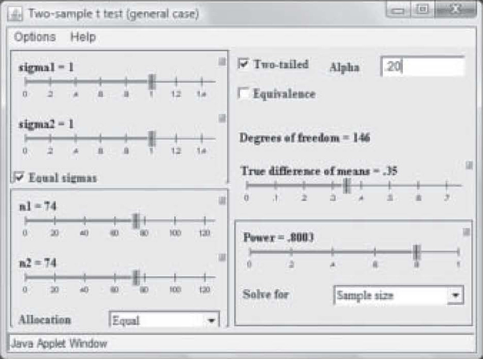
Figure 5. Sample size change due to change in alpha level.
A Type II error is less likely to be discovered than a Type I error. This is because when a Type II error is made, the conclusion is that there is no effect. Therefore, the line of research may be abandoned. With a Type I error, it is quite likely that other researchers will test the effect reported. When a number of them fail to find an effect, the original Type I error will be recognized. As noted, the probability of a Type I error is equal to the significance level of the study. What then, is the probability of a Type II error? That probability is calculated as 1-β. Since power is most often set at 0.80, the usual probability of a Type II error is 1– 0.80 or 0.20. Thus, while there is usually only a 5% chance of a Type I error, there is typically a 20% probability of a Type II error.
The statistic
The secondary factor that affects power is the statistic used. Each statistic has an associated power level. Parametric statistics are inherently more powerful than non-parametric statistics, but this is true only when they are used correctly. Non-parametric statistics are inherently less powerful than parametric statistics, but that is true only if the data and research methods used to acquire the data support the use of parametric statistics.
Parametric statistics are associated with a number of assumptions about the data. When those assumptions are violated, the parametric statistics become unstable and may provide misleading results. Assumptions of parametric statistics most commonly include the following: interval or ratio level of measurement of at least the dependent variable, random assignment of subjects to study group, random sampling from the population of interest, equal variances among the study groups for the dependent variable, and other related assumptions. These assumptions are based on the fact that parametric statistics are usually founded in the least squares formula, which uses the mean as the basis for calculation. When the mean is not an appropriate measure of central tendency for the data, non-parametric (or distribution-free) statistics should be used to test the hypotheses. Non-parametric statistics usually use the median or rank order of the data as the basis of their calculation. They therefore have far fewer assumptions than parametric statistics.
When the researcher inappropriately uses parametric statistics to test data which are not appropriate for parametric statistics, the power of the results is called into question. The author has personally seen a number of cases in which parametric statistics used on ordinal data failed to find a significant effect but the non-parametric statistic did find a significant effect. The converse is also true. An appropriately applied parametric statistic, being more powerful, found a significant treatment effect that the analogous non-parametric statistic did not find. For power to be adequate in a study, it is essential that the researchers use statistics appropriate to the data for hypothesis testing.
Conclusion
Power is primarily a function of sample size, effect size and alpha-level, and secondarily of the statistic used to test sample differences. The factor most readily manipulated by the researcher is the sample size. Power analysis has as its primary function the determination of the sample size necessary to achieve statistical significance in a study. However, power can also be used in pilot tests to identify treatment effects too weak to be worth further pursuit, and to identify the ideal significance level to be used in the main study. There are a number of power analysis calculators available on the Internet and the use of these calculators can provide a useful tool to researchers planning studies. They should always be used to identify the necessary sample size prior to beginning a study. A number of problems with interpretation of research results can be encountered if the researcher does not understand statistical power and how it is achieved. These include wrong interpretation of results due to either very low or very high power, and to inappropriate selection of a statistic to test the hypotheses. However, when power is adequate and the statistics are appropriately applied in hypothesis testing, the likelihood of correct conclusions is greatly improved.