Introduction
In order to choose the right statistical test, when analyzing the data from an experiment, we must have at least:
a decent understanding of some basic statistical terms and concepts;
some knowledge about few aspects related to the data we collected during the research/experiment (e.g. what types of data we have - nominal, ordinal, interval or ratio, how the data are organized, how many study groups (usually experimental and control at least) we have, are the groups paired or unpaired, and are the sample(s) extracted from a normally distributed/Gaussian population);
a good understanding of the goal of our statistical analysis;
we have to parse the entire statistical protocol in an well structured - decision tree /algorithmic manner, in order to avoid some mistakes.
The following questions and answers, will present, step by step, the terms and concepts necessary to realize this goal.
Question 1: What are the required basic terms and concepts?
Answer 1: Inference is the act or process of deriving a logical consequence conclusion from premises.
Statistical inference or statistical induction comprises the use of statistics and (random) sampling to make inferences concerning some unknown aspect of a statistical population (1,2).
It should be differentiated from descriptive statistics (3), which is used to describe the main features of data in quantitative terms (e.g. using central tendency indicators for the data – such as mean, median, mode or indicators of dispersion - sample variance, standard deviation etc). Thus, the aim of descriptive statistics is to quantitatively summarize a data set, opposed to inferential/inductive statistics, which is being used to support statements about the population that the data are thought to represent.
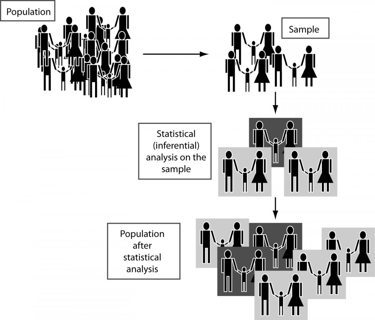
By using inferential statistics, we try to make inference about a population from a (random) sample drawn from it or, more generally, about a random process from its observed behavior during a finite period of time, as it can be seen in the following figure (Figure 1).
Figure 1. Using statistical analysis on sample(s) to make inferences about a population
Statistical inference may include (3, 4):
1. Point estimation, involving the use of sample data to calculate a single value (also known as a statistic), which is to serve as a “best guess” for an unknown (fixed or random) population parameter (e.g. relative risk RR = 3.72).
2. Interval estimation is the use of sample data to calculate an interval of possible (or probable) values of an unknown population parameter, in contrast to point estimation, which is a single number (e.g. confidence interval 95% CI for RR is 1.57-7.92).
We have to understand that sometime it is possible to use both, point and interval estimation, in order to make inferences about a parameter of the population through a sample extracted from it.
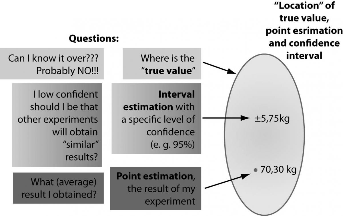
If we define the “true value” as the actual population value that would be obtained with perfect measuring instruments and without committing error of any type, we will have to accept that we may never know the true value of a parameter of the population (4). But, using the combination of these two estimators, we may obtain a certain level of confidence, that the true value may be in that interval, even if our result (point estimation) is not necessarily identical with the true value, as is illustrated in the figure below (Figure 2).
Figure 2. The concept of true value, point estimation and confidence interval
3. Prediction/forecast - forecasting is the process of estimation in unknown situations. A prediction is a statement or claim that a particular event will occur in the future in more certain terms than a forecast, so prediction is a similar, but more general term. Risk and uncertainty are central to forecasting and prediction.
4. Statistical hypothesis testing - last but not least, probably the most common way to do statistical inference is to use a statistical hypothesis testing. This is a method of making statistical decisions using experimental data and these decisions are almost always made using so-called “null-hypothesis” tests.
The null hypothesis (H0) formally describes some aspect of the statistical behavior of a set of data and this description is treated as valid unless the actual behavior of the data contradicts this assumption.
Because of this, the null hypothesis is contrasted against another hypothesis, so-called “alternative hypothesis” (H1). Statistical tests actually test the null hypothesis only. The null hypothesis test takes the form of: “There is no difference among the groups” for difference tests and “There is no association” for correlation tests. One can never “prove” the alternative hypothesis. One can only either reject the null hypothesis (in which case we accept the alternative hypothesis), or accept the null hypothesis.
It is important to understand that most of the statistical protocols used in current practice include one or more tests involving statistical hypothesis.
Question 2: Why do we need statistical inference and its principal exponent – statistical hypothesis testing?
Answer 2: In a few words, because we need to demonstrate in a scientific manner that, for example, an observed difference between the means of a parameter measured during an experiment involving two samples, is “statistically significant” (4).
A “statistically significant difference” simply means there is statistical evidence that there is a difference; it does not mean the difference is necessarily large, important, or significant in terms of the utility of the finding. It simply means that there is a measurable probability that the sample statistics are good estimates of the population parameters.
For a better understanding of the concept, let’s take an example. We took two samples of human subjects – a test sample, which received a treatment and a modified diet, and a control sample, which received placebo and a regular diet. For both samples, the body temperature and weight were recorded. The results from the experiment are presented in table 1.
If we will look at the results, based on “algebraic reasoning” we might say that there is a larger difference between the means of weight for those samples, than between the means of body temperature. But when we apply an appropriate statistical test for comparison between means (in this case, the appropriate test is “t-test for unpaired data”), the result will be surprising. The only statistically significant difference is between the means of body temperature, exactly the opposite conclusion that the one expected by our general knowledge and experience.
It becomes clear that we need statistical (significance) tests, in order to conclude that something has or hasn’t achieved “statistical significance“. Neither statistical nor scientific decisions can be reliably based on the judgment of “human eyes” or an observer’s “previous experience(s)”!
It must be noted that the researcher cannot be 100% sure about an observed difference, even when statistically significant. To deal with the level of “uncertainty” in such situations, two, let’s say “complementary”, key concepts of inferential statistics are introduced: confidence (C) (e.g. as in confidence intervals) and significance level (α - alpha) (5).
In simple terms, significance level (α, or alpha), may be defined as the probability of making a decision to reject the null hypothesis when the null hypothesis is actually true (a decision known as a Type I error, or “false positive determination”). Popular levels of significance are 5%, 1% and 0.1%, empirically corresponding to a “confidence level” of 95%, 99% and 99.9%.
Table 1. The results from the experiment
To a better understanding of these two terms, let’s take a general example. If the point estimate of a parameter is P, with confidence interval [x, y] at confidence level C, then any value outside the interval [x, y] will be significantly different from P at significance level α = 1 − C, under the same distributional assumptions that were made to generate the confidence interval.
That is to say, if in an estimation of a second parameter, we observed a value less than x or greater than y, we would reject the null hypothesis. In this case, the null hypothesis is: “the true value of this parameter equals P”, at the α level of significance; and conversely, if the estimate of the second parameter lay within the interval [x, y], we would be unable to reject the null hypothesis that the parameter equaled P.
Question 3: What steps are required to apply a statistical test?
Answer 3:
1. The statement of relevant null and alternative hypotheses to be tested.
2. Choosing significance level (represented by the Greek symbol α (alpha). Popular levels of significance are 5%, 1% and 0.1%, corresponding to a value of 0.05, 0.01 and 0.001 for α (alpha).
3. Compute the relevant test’s statistics (S), according with correct mathematical formula of the test.
4. Compare the test’s statistic (S) to the relevant critical values (CV) (obtained from tables in standard cases). Here we may obtain so-called “P value”.
5. Decide to either “fail to reject” the null hypothesis or reject it in favor of the alternative hypothesis. The decision rule is to reject the null hypothesis (H0) if S > CV and vice versa. Practically, if P ≤ α, we will reject the null hypothesis; otherwise we will accept it (4).
If we use modern statistical software, steps 3 and 4 are transparently done by the computer, so we may obtain directly the “P value”, avoiding the necessity to consult large statistical tables. Most statistical programs provide the computed results of test statistics.
Finally when we apply a statistical significance test to data from an experiment, we obtain a so-called “P-value”, which expresses the probability of having observed our results as extreme or even more extreme when the null hypothesis is true (6).
If we return to our example, illustrated in the table 1, the P value answers this question (7). If the populations from which those two samples were extracted, really did have the same mean, what is the probability of observing such a large difference (or larger) between sample means in an experiment when samples are of this size?
Thereby, if the P-value is 0.04, that means that there is a 4% chance of observing a difference as large as we observed when the two population means are actually identical (the null hypothesis is true). It is tempting to conclude, therefore, that there is a 96% chance that the difference we observed reflects a real difference between populations and a 4% chance that the difference is due to chance. This is a wrong conclusion. What we can say is that random sampling from identical populations would lead to a difference smaller than we observed (that is, the null hypothesis would be retained) in 96% of experiments and approximately equal to or larger than the difference we observed in 4% of experiments.
Choosing the right statistical test. What do we need to know before we start the statistical analysis?
Question 4: What type(s) of data may we obtain during an experiment?
Answer 4: Basic data collected from an experiment could be either quantitative (numerical) data or qualitative (categorical) data, both of them having some subtypes (4).
The quantitative (numerical) data could be:
1. Discrete (discontinuous) numerical data, if there are only a finite number of values possible or if there is a space on the number line between each 2 possible values (e.g. records from an obsolete mercury based thermometer).
2. Continuous data, that makes up the rest of numerical data, which could not be considered discrete. This is a type of data that is usually associated with some sort of advanced measurement using state of the art scientific instruments.
More importantly, the data may be measured at either an interval or ratio level. For the purposes of statistical analysis, the difference between the two levels of measurement is not important.
1. Interval data - interval data do not have an absolute zero and therefore it makes no sense to say that one level represents twice as much as that level if divided by two. For example, although temperature measured on the Celsius scale has equal intervals between degrees, it has no absolute zero. The zero on the Celsius scale represents the freezing point of water, not the total absence of temperature. It makes no sense to say that a temperature of 10 on the Celsius scale is twice as hot as 5.
2. Ratio data - ratio data do have an absolute zero. For example, when measuring length, zero means no length, and 10 meters is twice as long as 5 meters.
Both interval and ratio data can be used in parametric tests.
The qualitative (categorical) data could be:
1. Binary (logical) data - a basic type of categorical data (e.g. positive/negative; present/absent etc).
2. Nominal data - on more complex categorical data, the first (and weakest) level of data is called nominal data. Nominal level data is made up of values that are distinguished by name only. There is no standard ordering scheme to this data (e.g. Romanian, Hungarian, Croatian groups of people etc.).
3. Ordinal (ranked) data - the second level of categorical data is called ordinal data. Ordinal data are similar to nominal data, in that the data are distinguished by name, but different than nominal level data because there is an ordering scheme (e.g. small, medium and high level smokers).
Question 5: How could be these data types organized, before starting a statistical analysis?
Answer 5: Raw data is a term for data collected on source which has not been subjected to processing or any other manipulation (primary data) (4).
Thus, primary data is collected during scientific investigations, which need to be transformed into some format that allows interpretation and analysis between the variables.
Usually, the data from an experiment are collected using either a database managements system (Microsoft Access, Oracle, MySQL or even dedicated e-health record systems) or spreadsheet software (such as Microsoft Excel or OpenOffice Calc). In both cases, to be ready for statistical analysis, research data must be exported to a program that allows working with the data. They must be organized in a tabular (spreadsheet-like) manner using tables with an appropriate number of rows and columns, a format used by the majority of statistical packages.
If we have to deal with numerical data, those data can be organized in two ways, depending of the requirements of the statistical software we will use:
1. Indexed data – when we will have at least two columns: a column will contain the numbers recorded during the experiment and another column will contain the “grouping variable”. In this manner, using only two columns of a table we may record data for a large number of samples. Such approach is used in well known and powerful statistical software, such as SPSS (developed by SPSS Inc., now a division of IBM) and even in free software like Epiinfo (developed by Center for Disease Control - http://www.cdc.gov/epiinfo/downloads.htm) or OpenStat (developed by Bill Miller,http://statpages.org/miller/openstat/).
2. Raw data – when data are organized using a specific column (row) for every sample we may have. Even if this approach may be considered more intuitive from the beginner’s viewpoint, it is used by a relative small number of statistical software (e.g. MS Excel Statistics Add-in, OpenOffice Statistics or the very intuitive Graphpad Instat and Prism, developed by Graphpad Software Inc.).
If our recorded data are qualitative (categorical) data, the primary data table should be aggregated in a contingency table. A contingency table is essentially a display format used to analyze and record the relationship between two or more categorical variable. Basically, there are two types of contingency tables: “2 x 2” (tables with 2 rows and 2 columns) and “N x N” (where N > 2).
Question 6: How many samples may we have?
Answer 6: Depending on the research/study design, we may have three situations (4,7):
one sample;
two samples;
three or more samples.
If we have only one sample, we may ask a pertinent question: what statistical inference could be made, because no obvious comparison terms seem to be available?
Even if it looks like a dilemma, still some statistical analysis may be done. For example, if we administer a pyrogenic drug to one sample of laboratory animals, we still may be able to make some comparisons between the mean of body temperature recorded during the experiment and a well-known “normal” value for that species of animals, in order to demonstrate if the difference between those values has “statistical significance” and to conclude if the drug has or has not some pyrogenic effects.
If there are two samples involved in the research (this is one of the most common situations), all we have to do is to follow the proper protocol of inferential statistics to make the convenient comparisons between samples.
When more than two samples are involved, the analysis seems to be a little more complicated, but there are statistical tests available, more than capable to deal with such data. For example, we can make comparisons of means for all samples in one instance using analysis of variance (ANOVA test).
Also, we have to know that some post hoc tests are available, used if the null hypothesis is rejected at the second stage of the analysis of variance and able to make comparison between each and every pair of samples from the experiment.
Question 7: Do we have dependent or independent samples/paired or unpaired groups?
Answer 7: In general terms, whenever a subject in one group (sample) is related to a subject in the other group (sample), the samples are defined as “paired”.
For example, in a study of mothers and daughters, the samples are paired, a mother with her daughter. Subjects in the two samples are not independent of each other. For independent samples, the probability of a member of the population being selected is completely independent of any other subject being selected, either in the subject’s own group or in any other group in the study (7).
Paired data may be defined as values which fall normally into pairs and can therefore be expected to vary more between pairs than within pairs. If such conditions aren’t met, we will have to deal with unpaired or independent samples.
Why is this so important? Because there are many statistical tests that have different versions for paired/unpaired samples, with a different mathematical approach which may lead to different results. For example, a well-known statistical test, the t-test used for comparison of means between two samples, has different versions for paired/unpaired samples: paired (dependent) samples t-test and unpaired (independent) samples t-test.
Thereby, choosing a paired test (test for dependent samples) instead of an unpaired test (test for independent sample) is a mistake and may lead to wrong results/conclusions in the statistical inference process.
We have to choose a paired test when the experiment follows one of these designs (7):
when we measure a variable before and after an intervention in each subject;
when we recruit subjects as pairs, matched for variables such as age, ethnic group or disease severity - one of the pair gets one treatment; the other gets an alternative treatment;
when we run a laboratory experiment several times, each time with a control and treated preparation handled in parallel;
when we measure an outcome variable in child/parent pairs (or any other type of related pairs.
Broadly speaking, whenever we expect a value in one sample to be closer to a particular value in the other sample, than to a randomly selected value in the other sample, we have to choose a paired test, otherwise we choose an independent samples test.
Question 8: Are the data sampled from a normal/Gaussian distribution(s)?
Answer 8: Based on the normality of distributions, we chose parametric or nonparametric tests.
We should know that many statistical tests (e.g. t-tests, ANOVA and its variants), a priori assume that we have sampled data from populations that follow a Gaussian (normal/bell-shaped) distribution. Tests that follow this assumption, are called parametric tests and the branch of statistical science that uses such tests is called parametric statistics (4).
Parametric statistics assume that data come from a type of probability distribution (e.g. normal distribution) and make inferences about the parameters of the distribution. However, many populations from which data are measured - and biological data are often in this category - never follow a Gaussian distribution precisely. A Gaussian distribution extends infinitely in both directions and so includes both infinitely low negative numbers and infinitely high positive numbers and biological data are often naturally limited in range. Still, many kinds of biological data do follow a bell-shaped that is approximately Gaussian.
Thus, ANOVA tests, t-tests and other statistical tests work well, even if the distribution is only approximately Gaussian (especially with large samples, e.g. > 100 subjects) and these tests are used routinely in many fields of science.
But in some situations, for example when we have to deal with small samples (e.g. < 10) or have as an outcome variable a medical score (e.g. Apgar Score), applying such a test that assumes that the population follows a normal distribution, without a proper knowledge of the phenomena, could result in a P-value that may be misleading.
For this reason, another branch of statistics, called nonparametric statistics, propose distribution-free methods and tests, which do not rely on assumptions that the data are drawn from a given probability distribution (in our case, the normal distribution). Such tests are named nonparametric statistical tests (4). We should be aware that almost every parametric statistical test has a correspondent nonparametric test.
Maybe one of the most difficult decisions when we go through a statistical protocol is to choose between a parametric or nonparametric test. A pertinent question we may ask is the following one: if the nonparametric tests do not rely on assumptions that the data are drawn from normal distribution, why not use only such type of tests, to avoid a mistake?
To understand the difference between these two types of tests, we have to understand two more basic concepts in statistics: robustness and power of a statistical test.
A robust statistical test is one that performs well enough even if its assumptions are somewhat violated. In this respect, nonparametric tests tends to be more robust than their parametric equivalents, for example by being able to deal with very small samples, where data are far to be normally distributed.
The power of a statistical test is the probability that the test will reject the null hypothesis when the alternative hypothesis is true (e.g. that it will not make a type II error). As already previously extensively reviewed by Ilakovac (6), a Type II error is also known as an “error of the second kind”, a β error, or a “false negative” and is defined as the error of failing to reject a null hypothesis when it is in fact not true. As power increases, the chances of a Type II error decrease. Nonparametric tests tend to be more robust, but usually they have less power. In other words, a larger sample size can be required to draw conclusions with the same degree of confidence (7).
Question 9: When may we choose a proper nonparametric test?
Answer 9: We should definitely choose a nonparametric test in situations like these (7):
The outcome variable is a rank or score with fewer than a dozen or so categories (e.g. Apgar score). Clearly the population cannot be Gaussian in these cases.
The same problem may appear when the sample size is too small (< 10 or so).
When a few values are off scale, too high or too low to measure with a specific measurement technique. Even if the population is normally distributed, it is impossible to analyze the sample data with a parametric test (e.g. t-test or ANOVA). Using a nonparametric test with these kinds of data is easy because it will not rely on assumptions that the data are drawn from a normal distribution. Nonparametric tests work by recoding the original data into ranks. Extreme low and extreme high values are assigned a rank value and thus will not distort the analysis as would use of the original data containing extreme values. It won’t matter that a few values were not able to be precisely measured.
When we have enough “statistical confidence” that the population is far from normally distributed. A variety of “normality tests” are available to test the sample data for normal distribution.
Normality tests are used to determine whether a data set is well-modeled by a normal distribution or not. In other words, in statistical hypothesis testing, they will test the data against the null hypothesis that it is normally distributed.
The most common examples of such tests are:
1. D’Agostino-Pearson normality test – which computes the skewness and kurtosis to quantify how far from normality the distribution is in terms of asymmetry and shape. It then calculates how far each of these values differs from the value expected with a normal distribution, and computes a single P-value from the sum of these discrepancies. It is a versatile and powerful (compared to some others) normality test, and is recommended by some modern statistical books.
2. Kolmogorov-Smirnov test – used often in the past - compares the cumulative distribution of the data with the expected cumulative normal distribution, and bases its p-value simply on the largest discrepancy, which is not a very sensitive way to assess normality, thus becoming obsolete.
3. Beside of these two, there are a relatively large number of other normality tests, such as: Jarque-Bera test, Anderson-Darling test, Cramér-von-Mises criterion, Lilliefors test for normality (itself an adaptation of the Kolmogorov-Smirnov test),Shapiro-Wilk test, the Shapiro–Francia test for normality etc.
Using normality tests seems to be an easy way to decide if we will have to use a parametric or a non-parametric statistical test. But it is not, because we should pay attention to the size of the sample(s) before using such tests. For small samples (e.g. < 15), normality test are not very useful. They have little power to discriminate between Gaussian and non-Gaussian populations. Small samples simply do not contain enough information to let us make inferences about the shape of the distribution of the entire population. The table below will summarize the above discussion in a straightforward manner (Table 2).
Table 2. Parametric versus nonparametric tests
If the data do not follow a Gaussian (normal) distribution, we may be able to transform the values to create a Gaussian distribution (4). It is not the subject of this paper how this could be done, but, as a good example, for measurements (numerical data) one simple way to do this is to use logarithmic transformation: new value = log (old value).
In some cases, such a simple approach may permit us to use a parametric statistical test instead of a nonparametric one.
Question 10: Shall we choose one-tailed or two-tailed tests?
Answer 10: Let’s imagine that we design some studies/experiments to compare the height of young male adults (18-35 years) between various countries in the world (e.g between Sweden and South Korea and another, between Romania and Bulgaria). So, during a statistical analysis, a null hypothesis H0 (e.g. there is not a difference between the heights mean for those two independent samples) and an alternative hypothesis H1 for the specific statistical test has been formulated. Let’s consider that the distribution is Gaussian and the goal is to perform a specific test to determine whether or not the null hypothesis should be rejected in favor of the alternative hypothesis (in this case t-test for unpaired/independent samples will be the relevant one).
But there are two different types of tests that can be performed (4,7).
A one-tailed test looks only for an increase or a decrease (a one-way change) in the parameter whereas a two-tailed test looks for any change in the parameter (which can be any change - increase or decrease).
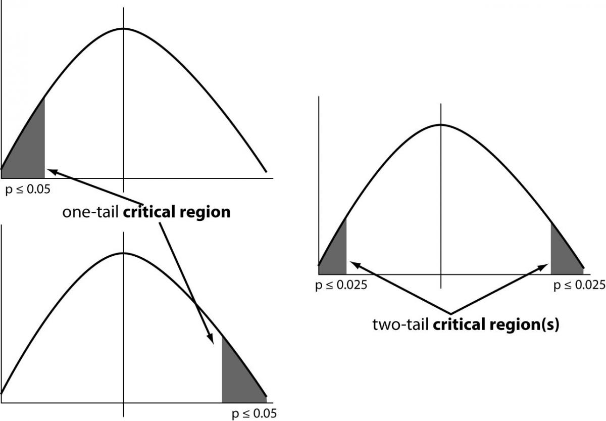
To understand this concept we have to define the critical region of a hypothesis test: the set of all outcomes which, if they occur, will lead us to decide to reject the null hypothesis in favor of the alternative hypothesis.
In a one-tailed test, the critical region will have just one part (the grey area in the figure below). If our sample value lies in this region, we reject the null hypothesis in favor of the alternative one. In a two-tailed test, we are looking for either an increase or a decrease. In this case, therefore, the critical region has two parts, as in figure 3.
Figure 3. Critical regions in one-tailed and two-tailed tests
When comparing two groups, we must distinguish between one- and two-tail P-values. The two-tail P-value answers this question: Assuming the null hypothesis is true, what is the chance that randomly selected samples would have means as far apart (or further) as we observed in this experiment with either group having the larger mean?
To interpret a one-tail P-value, we must predict which group will have the larger mean before collecting any data. The one-tail P-value answers this question: Assuming the null hypothesis is true, what is the chance that randomly selected samples would have means as far apart (or further) as observed in this experiment with the specified group having the larger mean?
A one-tail P-value is appropriate only when previous data, physical limitations or common sense tell us that a difference, if any, can only go in one direction. Or alternatively, we may be interested in a result only in one direction. For example, if a new drug has been developed to treat a condition for which an older drug exists. Clearly, researchers are only interested in continuing research on the new drug if it performs better than the old drug. The null hypothesis will be accepted if the new drug performs the same or worse than the older drug.
So, the real issue here is whether we have sufficient knowledge of the experimental situation to know that differences can occur in only one direction, or we are interested only in group differences in both directions.
In the light of these things, considering the above mentioned studies, we may choose a one-tail test only when we compare the heights mean of adult males between Sweden and South Korea, because our common sense and experience tell us that a difference, if any, can only go in one direction (the adult male Sweden citizens should be taller than the South Korean citizens).
When we make the same analysis for Romanian and Bulgarian citizens, this presumption may not be accurate, so we will have to choose a two-tailed test.
We should only choose a one-tail P-value when two things are true:
first, we must have predicted which group will have the larger mean before we collect any data;
if the other group ends up with the larger mean - even if it is quite a bit larger - then we must attribute that difference to chance.
For all these reasons, especially for beginners, choosing the right two-tailed test instead of a one-tailed test is recommended, unless we have a good reason to pick a one-tailed P-value.
Question 11: What is the goal of our statistical analysis?
Answer 11: When using basic statistical analysis, we may have, at most, three main goals (4,7):
1. To compare means (or medians) of the one, two or more groups/samples (e.g. is blood pressure higher in control than treated group(s)?).
2. To make some correlation, to look at how one or more independent variable(s) and one dependent variable relate to each other (e.g. how do weight and/or age affect blood pressure).
3. To measure association between one or more independent variables (e.g. epidemiological risk factors) and one or more dependent variables (e.g. diseases). This is so-called analysis of contingency tables, where we may look at how independent variable(s) (e.g. smoke or higher levels of smoking) are associated with one or more dependent variable(s) (e.g. lung cancer and its various forms).
Even if there are three goals, we will here discuss only the first goal: the means comparison between one, two or more groups/samples. Depending on how many samples we have, our goal will be to provide a scientific response to the following questions:
For one group/sample: we’ve measured a variable in this sample and the mean is different from a hypothetical (“normal”) value. Is this due to chance? Or does it tell us that the observed difference is a significant one?
For two groups/samples: we’ve measured a variable in two groups, and the means (and/or medians) seem to be distinct. Is that due to chance? Or does it tell us the two groups are really different?
For three or more groups/samples: we’ve measured a variable in three or more groups, and the means (and/or medians) are distinct. Is that due to chance? Or does it tell us the groups are really different? Which groups are different from which other groups?
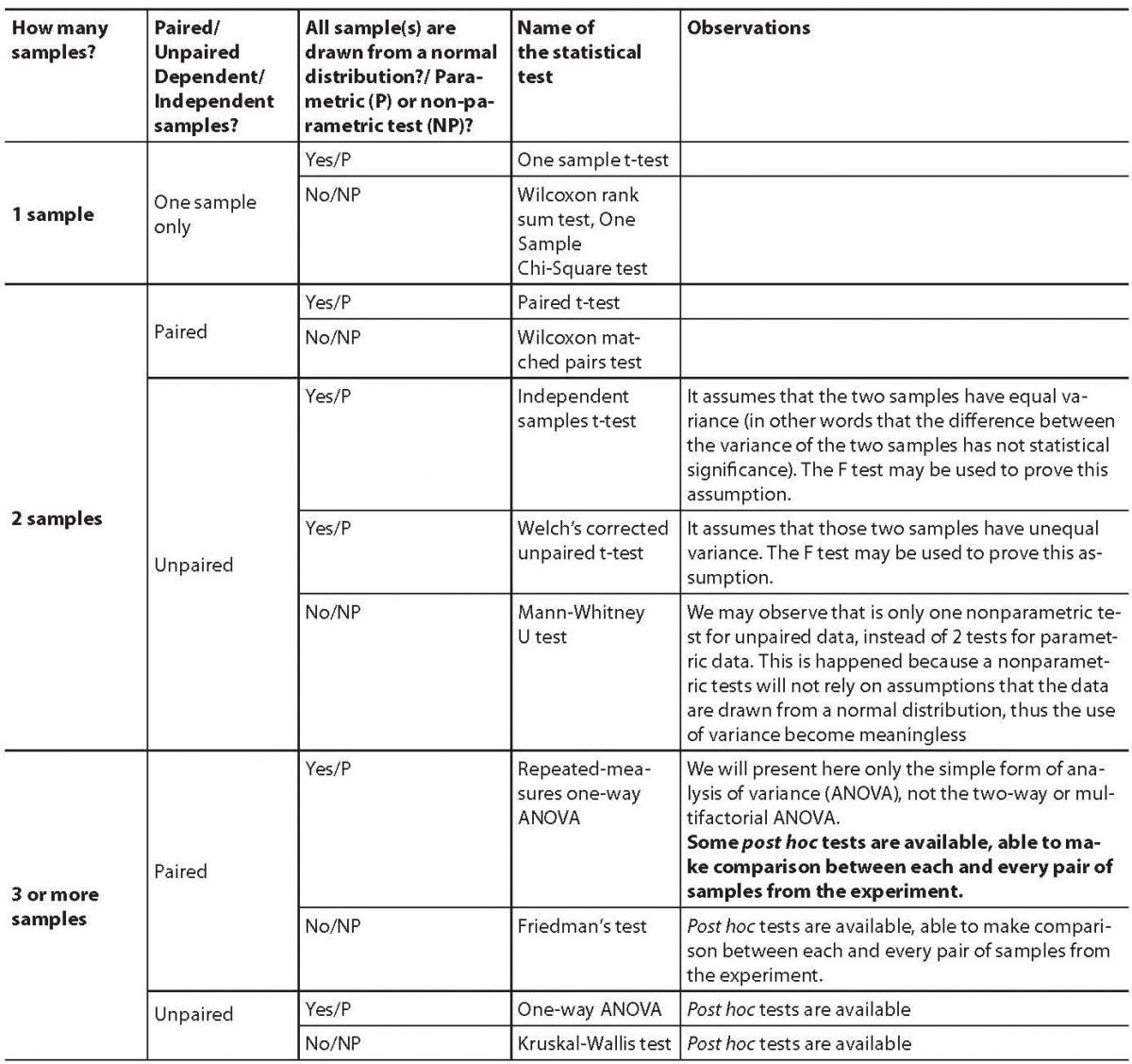
To provide a scientific response for such questions, we have to compare means (medians) of those groups/samples using one of the following statistical tests (with the recommendation to use a two-tailed test, unless we have a good reason to pick a one-tailed test) (Table 3).
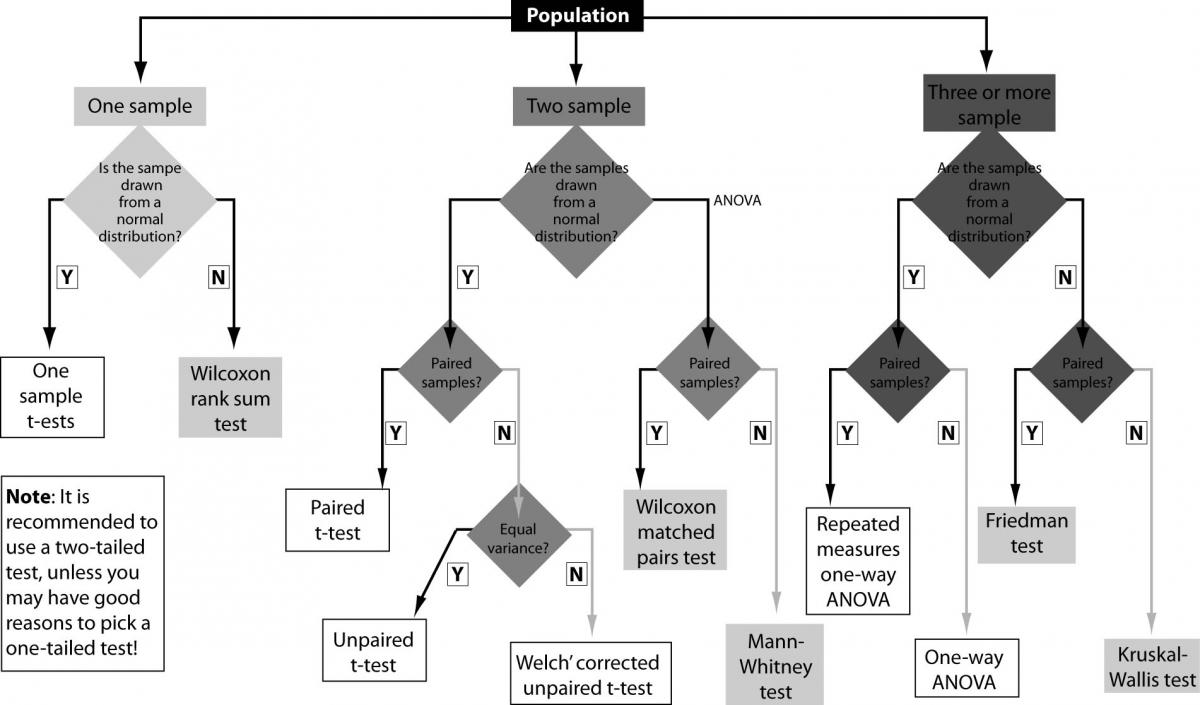
Now, knowing the basic terms and concepts, the tests selection process from the tests presented in the above table, can be very easy to understand if we shall think in an algorithmic manner, parsing the proper decision-tree, such as the one presented in the figure 4, to avoid any mistakes during the process.
Table 3. Statistical tests that compare the means (medians) for one, two, three or more groups/samples
Figure 4. The selection process for the right statistical test
Conclusion
The selection process of the right statistical test may be a difficult task, but a good knowledge and understanding of the proper statistical terms and concepts, may lead us to the correct decision.
We need, especially, to know what type of data we may have, how are these data organized, how many sample/groups we have to deal with and if they are paired or unpaired; we have to ask ourselves if the data are drawn for a Gaussian on non-Gaussian population and, if the proper conditions are met, to choose an one-tailed test (versus the two-tailed one, which is, usually, the recommended choice).
Based on such kind of information, we may follow a proper statistical decision-tree, using an algorithmic manner able to lead us to the right test, without any mistakes during the test selection process.
Even if we didn’t discussed here the means comparison when two or more factors are involved (e.g. bifactorial ANOVA) or the other two main goals of statistical inference (analysis of contingency tables and correlation/regression analysis), the algorithmic manner would be useful also in such cases, using the same approach to choose the right statistical test.
Still, some much disputed concepts will remain to be discussed in other future articles, such as outliers and their influence in statistical analysis, the impact of the missing data and so on.
