Introduction
The Chi-square test of independence (also known as the Pearson Chi-square test, or simply the Chi-square) is one of the most useful statistics for testing hypotheses when the variables are nominal, as often happens in clinical research. Unlike most statistics, the Chi-square (χ2) can provide information not only on the significance of any observed differences, but also provides detailed information on exactly which categories account for any differences found. Thus, the amount and detail of information this statistic can provide renders it one of the most useful tools in the researcher’s array of available analysis tools. As with any statistic, there are requirements for its appropriate use, which are called “assumptions” of the statistic. Additionally, the χ2 is a significance test, and should always be coupled with an appropriate test of strength.
The Chi-square test is a non-parametric statistic, also called a distribution free test. Non-parametric tests should be used when any one of the following conditions pertains to the data:
- The level of measurement of all the variables is nominal or ordinal.
- The sample sizes of the study groups are unequal; for the χ2 the groups may be of equal size or unequal size whereas some parametric tests require groups of equal or approximately equal size.
- The original data were measured at an interval or ratio level, but violate one of the following assumptions of a parametric test:
a) The distribution of the data was seriously skewed or kurtotic (parametric tests assume approximately normal distribution of the dependent variable), and thus the researcher must use a distribution free statistic rather than a parametric statistic.
b) The data violate the assumptions of equal variance or homoscedasticity.
c) For any of a number of reasons (1), the continuous data were collapsed into a small number of categories, and thus the data are no longer interval or ratio.
Assumptions of the Chi-square
As with parametric tests, the non-parametric tests, including the χ2 assume the data were obtained through random selection. However, it is not uncommon to find inferential statistics used when data are from convenience samples rather than random samples. (To have confidence in the results when the random sampling assumption is violated, several replication studies should be performed with essentially the same result obtained). Each non-parametric test has its own specific assumptions as well. The assumptions of the Chi-square include:
- The data in the cells should be frequencies, or counts of cases rather than percentages or some other transformation of the data.
- The levels (or categories) of the variables are mutually exclusive. That is, a particular subject fits into one and only one level of each of the variables.
- Each subject may contribute data to one and only one cell in the χ2. If, for example, the same subjects are tested over time such that the comparisons are of the same subjects at Time 1, Time 2, Time 3, etc., then χ2 may not be used.
- The study groups must be independent. This means that a different test must be used if the two groups are related. For example, a different test must be used if the researcher’s data consists of paired samples, such as in studies in which a parent is paired with his or her child.
- There are 2 variables, and both are measured as categories, usually at the nominal level. However, data may be ordinal data. Interval or ratio data that have been collapsed into ordinal categories may also be used. While Chi-square has no rule about limiting the number of cells (by limiting the number of categories for each variable), a very large number of cells (over 20) can make it difficult to meet assumption #6 below, and to interpret the meaning of the results.
- The value of the cell expecteds should be 5 or more in at least 80% of the cells, and no cell should have an expected of less than one (3). This assumption is most likely to be met if the sample size equals at least the number of cells multiplied by 5. Essentially, this assumption specifies the number of cases (sample size) needed to use the χ2 for any number of cells in that χ2. This requirement will be fully explained in the example of the calculation of the statistic in the case study example.
Case study
To illustrate the calculation and interpretation of the χ2 statistic, the following case example will be used:
The owner of a laboratory wants to keep sick leave as low as possible by keeping employees healthy through disease prevention programs. Many employees have contracted pneumonia leading to productivity problems due to sick leave from the disease. There is a vaccine for pneumococcal pneumonia, and the owner believes that it is important to get as many employees vaccinated as possible. Due to a production problem at the company that produces the vaccine, there is only enough vaccine for half the employees. In effect, there are two groups; employees who received the vaccine and employees who did not receive the vaccine. The company sent a nurse to every employee who contracted pneumonia to provide home health care and to take a sputum sample for culture to determine the causative agent. They kept track of the number of employees who contracted pneumonia and which type of pneumonia each had. The data were organized as follows:
- Group 1: Not provided with the vaccine (unvaccinated control group, N = 92)
- Group 2: Provided with the vaccine (vaccinated experimental group, N = 92)
In this case, the independent variable is vaccination status (vaccinated versus unvaccinated). The dependent variable is health outcome with three levels:
- contracted pneumoccal pneumonia;
- contracted another type of pneumonia; and
- did not contract pneumonia.
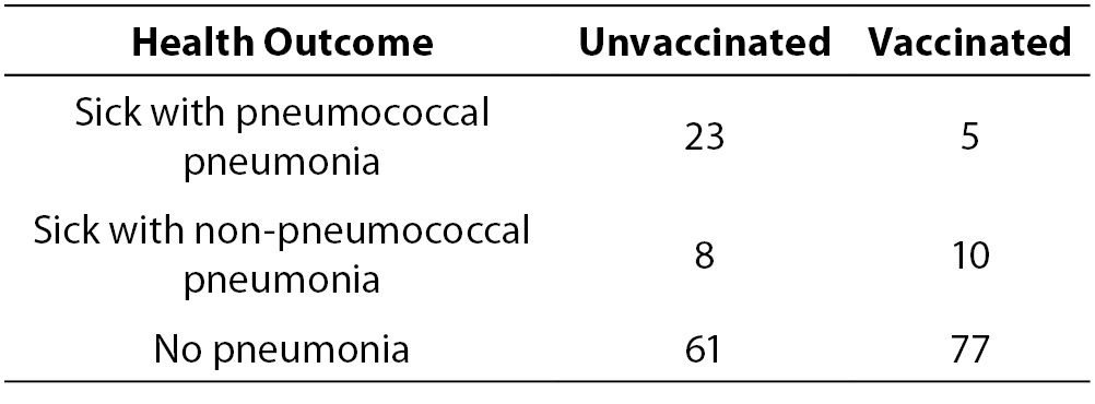
The company wanted to know if providing the vaccine made a difference. To answer this question, they must choose a statistic that can test for differences when all the variables are nominal. The χ2 statistic was used to test the question, “Was there a difference in incidence of pneumonia between the two groups?” At the end of the winter, Table 1 was constructed to illustrate the occurrence of pneumonia among the employees.
Table 1. Results of the vaccination program.
Calculating Chi-square
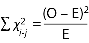
With the data in table form, the researcher can proceed with calculating the χ2 statistic to find out if the vaccination program made any difference in the health outcomes of the employees. The formula for calculating a Chi-Square is:
Where:
O = Observed (the actual count of cases in each cell of the table)
E = Expected value (calculated below)
χ2=The cell Chi-square value
=Formula instruction to sum all the cell Chi-square values
= i-j is the correct notation to represent all the cells, from the first cell (i) to the last cell (j); in this case Cell 1 (i) through Cell 6 (j).
The first step in calculating a χ2 is to calculate the sum of each row, and the sum of each column. These sums are called the “marginals” and there are row marginal values and column marginal values. The marginal values for the case study data are presented in Table 2.
Table 2. Calculation of marginals.
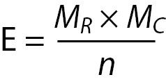
The second step is to calculate the expected values for each cell. In the Chi-square statistic, the “expected” values represent an estimate of how the cases would be distributed if there were NO vaccine effect. Expected values must reflect both the incidence of cases in each category and the unbiased distribution of cases if there is no vaccine effect. This means the statistic cannot just count the total N and divide by 6 for the expected number in each cell. That would not take account of the fact that more subjects stayed healthy regardless of whether they were vaccinated or not. Chi-Square expecteds are calculated as follows:
Where:
E = represents the cell expected value,
MR = represents the row marginal for that cell,
MC = represents the column marginal for that cell, and
n = represents the total sample size.
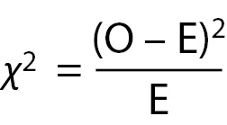
Specifically, for each cell, its row marginal is multiplied by its column marginal, and that product is divided by the sample size. For Cell 1, the math is as follows: (28 x 92)/184 = 13.92. Table 3 provides the results of this calculation for each cell. Once the expected values have been calculated, the cell χ2values are calculated with the following formula:
The cell χ2for the first cell in the case study data is calculated as follows: (23-13.93)2/13.93 = 5.92. The cell χ2value for each cellis the value in parentheses in each of the cells in Table 3.
Table 3. Cell expected values and (cell Chi-square values).
Once the cell χ2 values have been calculated, they are summed to obtain the χ2 statistic for the table. In this case, the χ2 is 12.35 (rounded). The Chi-square table requires the table’s degrees of freedom (df) in order to determine the significance level of the statistic. The degrees of freedom for a χ2table are calculated with the formula:
(Number of rows -1) x (Number of columns -1).
For example, a 2 x 2 table has 1 df. (2-1) x (2-1) = 1. A 3 x 3 table has (3-1) x (3-1) = 4 df. A 4 x 5 table has (4-1) x (5-1) = 3 x 4 = 12 df. Assuming a χ2value of 12.35 with each of these different df levels (1, 4, and 12), the significance levels from a table of χ2 values, the significance levels are: df = 1, P < 0.001, df = 4, P < 0.025, and df = 12, P > 0.10. Note, as degrees of freedom increase, the P-level becomes less significant, until the χ2 value of 12.35 is no longer statistically significant at the 0.05 level, because P was greater than 0.10.
For the sample table with 3 rows and 2 columns, df = (3-1) x (2-1) = 2 x 1 = 2. A Chi-square table of significances is available in many elementary statistics texts and on many Internet sites. Using a χ2 table, the significance of a Chi-square value of 12.35 with 2 df equals P < 0.005. This value may be rounded to P < 0.01 for convenience. The exact significance when the Chi-square is calculated through a statistical program is found to be P = 0.0011.
As the P-value of the table is less than P < 0.05, the researcher rejects the null hypothesis and accepts the alternate hypothesis: “There is a difference in occurrence of pneumococcal pneumonia between the vaccinated and unvaccinated groups.” However, this result does not specify what that difference might be. To fully interpret the result, it is useful to look at the cell χ2 values.
Interpreting cell χ2 values
It can be seen in Table 3 that the largest cell χ2 value of 5.92 occurs in Cell 1. This is a result of the observed value being 23 while only 13.92 were expected. Therefore, this cell has a much larger number of observed cases than would be expected by chance. Cell 1 reflects the number of unvaccinated employees who contracted pneumococcal pneumonia. This means that the number of unvaccinated people who contracted pneumococcal pneumonia was significantly greater than expected. The second largest cell χ2 value of 4.56 is located in Cell 2. However, in this cell we discover that the number of observed cases was much lower than expected (Observed = 5, Expected = 12.57). This means that a significantly lower number of vaccinated subjects contracted pneumococcal pneumonia than would be expected if the vaccine had no effect. No other cell has a cell χ2value greater than 0.99.
A cell χ2 value less than 1.0 should be interpreted as the number of observed cases being approximately equal to the number of expected cases, meaning there is no vaccination effect on any of the other cells. In the case study example, all other cells produced cell χ2 values below 1.0. Therefore the company can conclude that there was no difference between the two groups for incidence of non-pneumococcal pneumonia. It can be seen that for both groups, the majority of employees stayed healthy. The meaningful result was that there were significantly fewer cases of pneumococcal pneumonia among the vaccinated employees and significantly more cases among the unvaccinated employees. As a result, the company should conclude that the vaccination program did reduce the incidence of pneumoccal pneumonia.
Very few statistical programs provide tables of cell expecteds and cell χ2 values as part of the default output. Some programs will produce those tables as an option, and that option should be used to examine the cell χ2 values. If the program provides an option to print out only the cell χ2 value (but not cell expecteds), the direction of the χ2 value provides information. A positive cell χ2 value means that the observed value is higher than the expected value, and a negative cell χ2 value (e.g. -12.45) means the observed cases are less than the expected number of cases. When the program does not provide either option, all the researcher can conclude is this: The overall table provides evidence that the two groups are independent (significantly different because P < 0.05), or are not independent (P > 0.05). Most researchers inspect the table to estimate which cells are overrepresented with a large number of cases versus those which have a small number of cases. However, without access to cell expecteds or cell χ2 values, the interpretation of the direction of the group differences is less precise. Given the ease of calculating the cell expecteds and χ2 values, researchers may want to hand calculate those values to enhance interpretation.
Chi-square and closely related tests
One might ask if, in this case, the Chi-square was the best or only test the researcher could have used. Nominal variables require the use of non-parametric tests, and there are three commonly used significance tests that can be used for this type of nominal data. The first and most commonly used is the Chi-square. The second is the Fisher’s exact test, which is a bit more precise than the Chi-square, but it is used only for 2 x 2 Tables (4). For example, if the only options in the case study were pneumonia versus no pneumonia, the table would have 2 rows and 2 columns and the correct test would be the Fisher’s exact. The case study example requires a 2 x 3 table and thus the data are not suitable for the Fisher’s exact test.
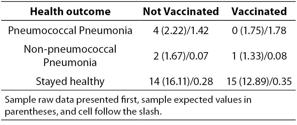
Table 4. Example of a table that violates cell expected values.
The third test is the maximum likelihood ratio Chi-square test which is most often used when the data set is too small to meet the sample size assumption of the Chi-square test. As exhibited by the table of expected values for the case study, the cell expected requirements of the Chi-square were met by the data in the example. Specifically, there are 6 cells in the table. To meet the requirement that 80% of the cells have expected values of 5 or more, this table must have 6 x 0.8 = 4.8 rounded to 5. This table meets the requirement that at least 5 of the 6 cells must have cell expected of 5 or more, and so there is no need to use the maximum likelihood ratio chi-square. Suppose the sample size were much smaller. Suppose the sample size was smaller and the table had the data in Table 4.
Although the total sample size of 39 exceeds the value of 5 cases x 6 cells = 30, the very low distribution of cases in 4 of the cells is of concern. When the cell expecteds are calculated, it can be seen that 4 of the 6 cells have expecteds below 5, and thus this table violates the χ2test assumption. This table should be tested with a maximum likelihood ratio Chi-square test.
When researchers use the Chi-square test in violation of one or more assumptions, the result may or may not be reliable. In this author’s experience of having output from both the appropriate and inappropriate tests on the same data, one of three outcomes are possible:
First, the appropriate and the inappropriate test may give the same results.
Second, the appropriate test may produce a significant result while the inappropriate test provides a result that is not statistically significant, which is a Type II error.
Third, the appropriate test may provide a non-significant result while the inappropriate test may provide a significant result, which is a Type I error.
Strength test for the Chi-square
The researcher’s work is not quite done yet. Finding a significant difference merely means that the differences between the vaccinated and unvaccinated groups have less than 1.1 in a thousand chances of being in error (P = 0.0011). That is, there are 1.1 in one thousand chances that there really is no difference between the two groups for contracting pneumococcal pneumonia, and that the researcher made a Type I error. That is a sufficiently remote probability of error that in this case, the company can be confident that the vaccination made a difference. While useful, this is not complete information. It is necessary to know the strength of the association as well as the significance.
Statistical significance does not necessarily imply clinical importance. Clinical significance is usually a function of how much improvement is produced by the treatment. For example, if there was a significant difference, but the vaccine only reduced pneumonias by two cases, it might not be worth the company’s money to vaccinate 184 people (at a cost of $20 per person) to eliminate only two cases. In this case study, the vaccinated group experienced only 5 cases out of 92 employees (a rate of 5%) while the unvaccinated group experienced 23 cases out of 92 employees (a rate of 25%). While it is always a matter of judgment as to whether the results are worth the investment, many employers would view 25% of their workforce becoming ill with a preventable infectious illness as an undesirable outcome. There is, however, a more standardized strength test for the Chi-Square.
Statistical strength tests are correlation measures. For the Chi-square, the most commonly used strength test is the Cramer’s V test. It is easily calculated with the following formula:
Where n is the number of rows or number of columns, whichever is less. For the example, the V is 0.259 or rounded, 0.26 as calculated below.
The Cramer’s V is a form of a correlation and is interpreted exactly the same. For any correlation, a value of 0.26 is a weak correlation. It should be noted that a relatively weak correlation is all that can be expected when a phenomena is only partially dependent on the independent variable.
In the case study, five vaccinated people did contract pneumococcal pneumonia, but vaccinated or not, the majority of employees remained healthy. Clearly, most employees will not get pneumonia. This fact alone makes it difficult to obtain a moderate or high correlation coefficient. The amount of change the treatment (vaccine) can produce is limited by the relatively low rate of disease in the population of employees. While the correlation value is low, it is statistically significant, and the clinical importance of reducing a rate of 25% incidence to 5% incidence of the disease would appear to be clinically worthwhile. These are the factors the researcher should take into account when interpreting this statistical result.
Summary and conclusions
The Chi-square is a valuable analysis tool that provides considerable information about the nature of research data. It is a powerful statistic that enables researchers to test hypotheses about variables measured at the nominal level. As with all inferential statistics, the results are most reliable when the data are collected from randomly selected subjects, and when sample sizes are sufficiently large that they produce appropriate statistical power. The Chi-square is also an excellent tool to use when violations of assumptions of equal variances and homoscedascity are violated and parametric statistics such as the t-test and ANOVA cannot provide reliable results. As the Chi-Square and its strength test, the Cramer’s V are both simple to compute, it is an especially convenient tool for researchers in the field where statistical programs may not be easily accessed. However, most statistical programs provide not only the Chi-square and Cramer’s V, but also a variety of other non-parametric tools for both significance and strength testing.
