Introduction
The more traditional, widespread and practiced method for interpreting the laboratory results is based on the comparison made with reference intervals. As defined by the International Federation of Clinical Chemistry (IFCC) (1), the terms “reference range” or “interval of reference” (IR) mean a range of values obtained from individuals (usually, but not necessarily healthy) randomly chosen, but appropriately selected in order to satisfy suitably defined criteria (2). The apparent contradiction between “random” and “appropriate selection” is resolved bearing in mind that these are two phases of the same process of identification of IR (3). Population based studies are preliminary steps for selecting the reference intervals, being numerous the variables that can affect the population characteristics (Table 1). It appears however very important to stress the fact that each laboratory should be able to establish the reference values that are as close as possible to those presented by the population who insists close to the operating lab itself. Of course, it is understandable that in the event of the introduction of new activities (new laboratory or new tests by any laboratory), as well as during transitional periods, provisional IR may be chosen, e.g. by opportunely adapting IRs from laboratories operating in nearby areas, as well as from reliable data in literature (4). However, the constraint should be of finding and setting own IRs as soon as possible. In this circumstance, we should think about the influence that the progressive aging of the population or the different gender distribution observed in different areas of the country have on some analysis (e.g., blood glucose, blood urea nitrogen, creatinine), or even more so the effects of immigration from countries very far or different each other.
Table 1. Preconditions for the formulation of a reference interval in healthy subjects.
IR establishment
The creation of reference intervals requires careful planning, monitoring and documentation of every aspect of the study. Consequently, the reference intervals must be well characterized in terms of variations attributable to the pre-analytical and analytical factors (5). These formal protocols are particularly useful in cases where a laboratory should establish its own reference range for a particular test. This situation can occur even if a laboratory has modified a test or a method approved and/or certified, or a method developed in-house. Unfortunately, these protocols are resource intensive and can be prohibitive for smaller facilities, also in consideration of the inherent costs (6). Even large laboratories may find it difficult to carry out these studies for obtaining their own IRs, mainly based on considerations of cost-benefit analysis. Thus many laboratories have increased their reliance on manufacturers to adopt reference intervals that may be acceptable using simpler approaches, which require less effort and result in lower costs. In any case, it is desirable that each laboratory has complete knowledge of the characteristics of the reference ranges adopted, such that they ensure compatibility with its own population and are suitable for clinical use.
An IR is usually determined by analyzing samples that are obtained from individuals who meet the criteria previously and accurately defined (reference sample group). Protocols such as those made by the “International Federation of Clinical Chemistry [IFCC] Expert Panel on Theory of Reference Values” and by the “National Committee for Clinical Laboratory Standards” show in a comprehensive and systematic manner the processes that use carefully selected reference sample groups to establish reference intervals. These protocols typically require a minimum of 120 reference persons for each group (or subgroup) to be characterized (7). However, it is increasingly gaining importance a vision that considers more appropriate to adopt reference intervals common to several laboratories that operate over large regional areas and also on entire national context (8–10).
When establishing reference intervals that are common to most laboratories in the same area, the sample size can be expanded considerably around the local production of reference intervals for each individual laboratory. When many laboratories can share common reference intervals, the investment is limited and the whole operation can advantageously be concentrated in one or a few institutions. Consequently, one can work on much larger sample sizes, such as five/six hundreds or more individuals. A larger sample makes it possible to carry out a thorough investigation of possible subgroups (11) in which it is possible to obtain reliable estimates on the reference intervals subgroup, respecting the minimum size of 120 individuals recommended by the IFCC. The confidence interval (CI) of 90% for a sample of similar size is Cl = ± 0.24 × SD (standard deviation of the population). The allocation criteria are (4):
If one or both; the difference between the lower reference limits and the difference between the higher reference limits of the two subgroups are > 0.75 × SDmin (where SDmin is the smallest DS of the subset of the DS), then the partition is recommended.
If both; the differences between the lower reference limits and the higher reference limits of both subgroups are ≤ 0.25 × SDmin, then the partition is not recommended.
For differences which fall between the extremes (0.25 × SDmin < difference < 0.75 × SDmin), the arguments should differ from the purely statistical ones, as this could be due to genetic differences, i.e. to situations which are not routinely assessed.
Selection of the reference population
The selection of the population who will represent the “reference” can not be dealt with in general terms, as more than one variable have to be considered. The most common method is to obtain reference values from a population of healthy individuals, but in this case the definition of “health” is indeed problematic. For example, to establish a reference interval for hemoglobin levels (i.e., a gender-related laboratory test), the laboratory would need to obtain the results of hemoglobin from at least 240 persons (120 men and 120 women). These people are usually drawn from the local population and then selected for inclusion in the study using carefully defined criteria. The general criteria that are adopted are those reported in Table 2; moreover there is the opportunity to use a series of strategies, assuming additional criteria of subdivision for subgroups (Table 3) and/or age (Table 4) or combine multiple criteria, as for example (4):
- Selection of homogeneous groups of reference according to ethnicity, geographical origin and environmental conditions in
order to obtain the representation of the population to which the normal range will apply.
- Stratification according to age and gender, if there are women pregnant or taking any anti-conceptional drug.
- Definition of health status, according to further criteria that are adopted.
Table 2. Exclusion criteria for the formulation of reference range in the general population.
Table 3. Criteria for the creation of subgroups of reference subjects.
Table 4. Reference intervals: Criteria for distributions in the different age group.
There are no particular recommendations on which method of selection is the most appropriate, as this may depend both on the purpose of the investigation, and on the opportunities allowing to include single individuals. In any case it is important to report the strategy adopted and the individuals included in the reference interval and to implement clear criteria for inclusion and exclusion.
Statistics
The normal or Gaussian distribution (Figure 1) is the distribution characterized by two parameters, mean and standard deviation (SD). The statistical methods that assume Gaussian distribution of data are called parametric methods. Of course, other probability distributions, whose characteristics are defined by one or more parameters, can be analyzed using appropriate parametric methods.
Figure 1. The normal or Gaussian distribution.
Non-parametric statistical techniques are used to analyze the data not having a specific type of probability distribution. In general, when observing non-Gaussian distributions (non-normal) (Figure 2a-b), their description is assigned to other indices such as median, percentiles classes, and more others. Moreover, in this second category of data distribution, other methods become more useful, including the so called and important ones “bootstrap methods”. Sometimes non-Gaussian distributions can be normalized via appropriate processing techniques (12). This is the general case of distributions obtained from experimental data, for which the assumption of normality is always verified. In constructing a reference range from individual data, often the difficulty of achieving a perfect Gaussian distribution is apparent. Even after sampling the data from a population which is presumed to be normally distributed, it is often necessary to take some approximations of the data to comply with the assumption of normality. In this regard a series of statistical tests have been put in place, which compares the distribution of experimental data with a hypothetical Gaussian distribution (13–15). These methods are called mathematical-statisticalgoodness-of-fit test tests. Among them, the most known and used is the Kolmogorov-Smirnov, although its real discriminant power is questioned by some researchers, especially when the parameters of the distribution are estimated based on data rather than being specified a priori. Afterwards, other tests have been proposed that are best suited for this purpose, among them the test of Shapiro-Wilks (for distribution of samples greater than 2,000 subjects it should be replaced by the test for normality of Stephen) and the test of D’Agostino-Pearson. None of these tests can however indicate the type of non-normalityobserved in the case where the distribution is showing tendency to asymmetry (skewness) and kurtosis or both (Figure 3).
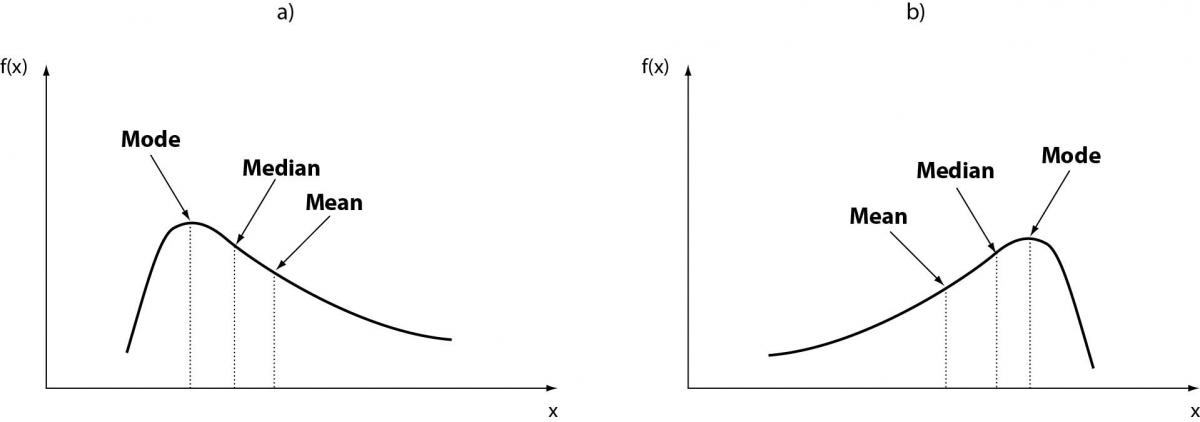
Figure 2. Non-Gaussian distribution (non-normal).
Figure 3. Tendency to asymmetry (skewness).
The skewness represents the degree of asymmetry of a distribution around its mean and is non-dimensional since it is characterized only by a number describing the shape of the distribution curve. When a distribution is perfectly Gaussian, the skewness score is equal to 0. Skewness figures more or less negative or positive (e.g., +2.0 or –1.5) correspond to a form of distribution curve with a tail more or less pronounced towards positive or negative values on the x axis. Similarly, the kurtosis represents the degree to which the peak of distribution is sharp or flat, fluctuating between +3 and –3. In a perfectly Gaussian curve the kurtosis score is 0 and of the distribution is called mesokurtic (Figure 4). Many mathematical functions to correct either the skewness or the kurtosis have been proposed, and in some cases recommended, but their application was generally marginal. In practice, since a certain degree of skewness is always observed, a rule of thumb has been defined according to which each distribution is considered Gaussian when the relationship between skewness and standard error is < ± 2. A similar exercise is suggested for the kurtosis, using the relationship between kurtosis and standard error of kurtosis. After ascertaining that the assumption of normality is not violated in a significant manner, the main parameters of the Gaussian curve (mean and standard deviation) are calculated and the interval of reference is considered to be comprised within the values of the mean ± 1.96 × standard deviation (sometimes 1.96 is rounded to 2.00) (Figure 5).
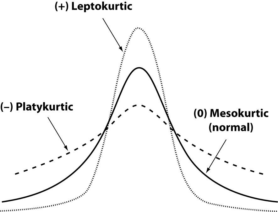
Figure 4. General forms of kurtosis.
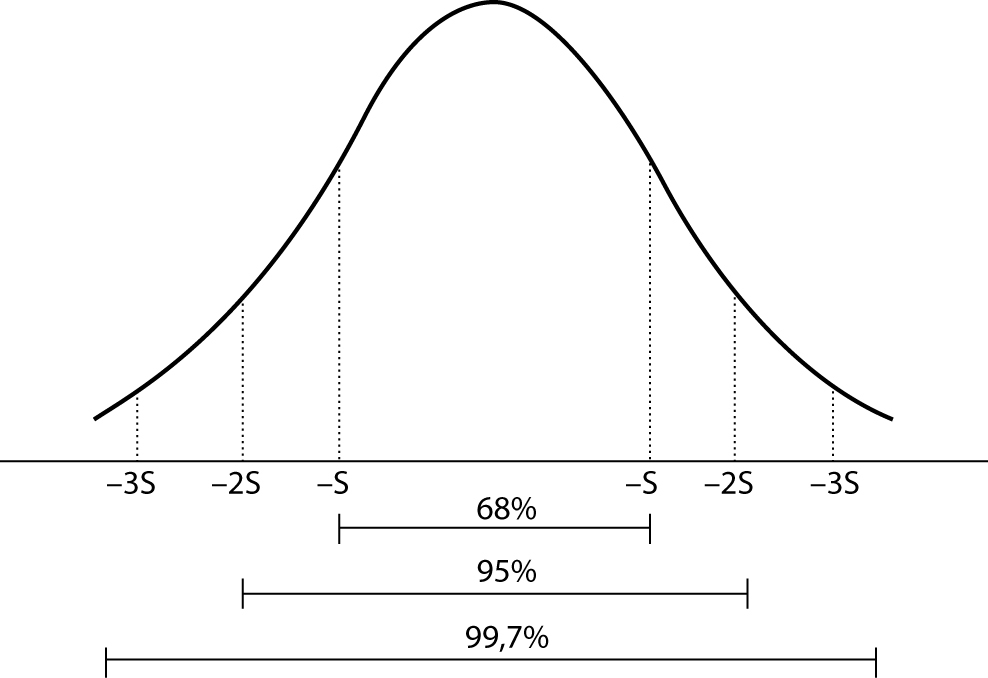 Figure 5. Interval of reference: Gaussian curve.
When the assumption of normality tests do not fit a normal curve, a logarithmic transformation of data can be used, in order to restore the data to a normal distribution curve; the above parameters (mean and SD) can be then calculated.
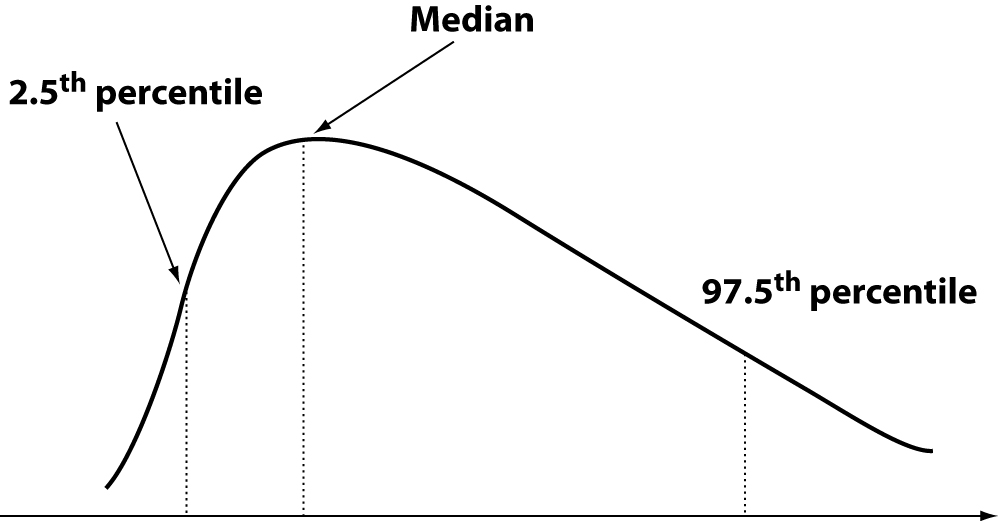
However, sometimes no transformation and/or processing of data is possible. This can happen with data from measures of analytes expressed by specific genes, such as highly polymorphic proteins (eg haptoglobin, lipoprotein (a)), homocysteine and others. To overcome these problems, the IFCC through its Expert Panel on Theory of Reference Values, has recommended the use of interpercentile intervals estimated on statistical methods either parametric or nonparametric, although the recommendation is in favour of the non-parametric approach (7). Although parametric methods are most commonly employed and seemingly simple from the point of view of calculations, they maintain unresolved all the problems outlined above. The nonparametric methods, though a bit less easy to set up, have the ability to largely avoid such problems. Many procedures have been described (16). Currently the preferred method is based on iterative bootstrap ranking (17). The target range is between the 2.5th and the 97.5 th percentile (Figure 6). Even in these cases the values below and above these limits are considered “out of normality”. A widely diffused but not supported by solid bases opinion is that the reference interval from Gaussian and non-Gaussian distributions represents the values of individuals to be referred to (i.e., “the normal individuals”) and that the areas at the “tails” of the curve represent individuals whose values are to be rejected as “out of normality.” This is a misconception, because (18):
1. Even these values come from individuals originally included in the group chosen according to the characteristics set out before the construction of the interval of reference.
2. All values, both central and those close to the limits of distribution, are only representations of biological variability on time.
3. In any case the analytical variability influences the current data.
The above concepts are well known to professionals in laboratories, but are largely ignored or underestimated in the clinical practice. Actually, the reference limits are not cut-off limits, because they are influenced by both the biological variability and the analytical one. Based on these considerations, the IFCC recommends estimating a confidence range of 90% for each limit of the reference interval in both Gaussian and non-Gaussian distribution.
Figure 6. Interpercentile intervals: nonparametric distribution.
Longitudinal comparison of laboratory results
The concept of change of reference (CR) was proposed by Harris and Yasaka to enable evaluation of the observed change between two successive measures (19). The longitudinal comparison is based on this concept and is mainly justified by the clinical problems that are not adequately answered by a cross-comparison based on the interval of reference. The Reference Change Value (or RCV) is especially useful in monitoring and follow-up of various clinical conditions. RCV is calculated by taking into account intra-individual biological variability, in addition to analytical variability in the medium to long term, in order to take into account the time elapsed between the test results. The general formula is as follows:
RCV = zp × 21/2 × (CVa + CVw)1/2;
where zp is the probability density function (generally 1.96 at P = 0.05), CVw is the intra-individual biological variability andCVa is the variability of analytical testing. RCV shows some special additional benefits to get information on the status of patients, particularly in the monitoring of clinically stable and well controlled conditions, such as the prognosis of the crisis of rejection in kidney transplant patients, monitoring of oral anticoagulant therapy (OAT), the glycated hemoglobin (A1c) in diabetes and other conditions (20–23). RCV is only applicable when CVa < 0.5 < CVw. Close monitoring of analytical quality is needed for, especially when the time between the first test and the next is rather long such as for glycated hemoglobin.
In discussing the comparison of longitudinal data it appears appropriate to introduce the concept of index of individuality (I.I.) (24,25). The I.I. represents the ratio of the random distribution of values observed in samples taken from one individual for a given test compared to the distribution of values of the entire population of individuals for the same test. When the observed I. I. is low, it is of little clinical utility using traditional reference interval. A cut-off value of I.I. ≤ 0.6 is considered and in this case the comparison of longitudinal data is much more suited to evaluate the changes observed using RCV. When the results of laboratory tests with a low RCV are located near the limits of distribution of the traditional IR, in a position of low frequency, there are two possibilities:
a) stable condition if the previous result was similar;
b) a condition achieved in recent times if the result show variation.
Since in this case the traditional IR is insensitive and therefore not needed, only a previous result of that test can clarify the situation. It is also important to consider that many of the laboratory tests that explore aspects of body metabolism show low homeostatic I.I. in respect of IR. For a number of tests it seems therefore important to collect the results in databases or systems for collecting personal data (such as chip-based flash memory card, now widely available and very inexpensive) to access when needed. For every repetition of the series of tests, the results should be collected, and compared to the previous ones.
Recently the concept of estimating the differences between serial results as the probability of change by calculating the likelihood ratio (likelihood ratio) in addition to RCV has been introduced (26). The procedure appears robust from a theoretical point of view and deserves to be widely adopted, as it seems likely to improve the monitoring of individual conditions and provide clinical support to rational clinical decision. Each individual could benefit from a progressive assessment (“in progress”) of their own health and any deviation from her/his reference state identified and assessed.
Conclusions
The quality performances resulting from the current technology advancements allow clinical laboratories to fully exploit the opportunity of creating common IRs in order to accomplish transferability of data, thus increasing citizens benefits and meeting health system expectations.
Notes
Potential conflict of interest
None declared.
References
1. Solberg HE. The IFCC recommendation on estimation of reference intervals. The RefVal program. Clin Chem Lab Med 2004;42:710-4.
2. Solberg HE, PetitClerc C. International Federation of Clinical Chemistry (IFCC), Scientific Committee, Clinical Section, Expert Panel on Theory of Reference Values. Approved recommendation (1987) on the theory of reference values. Part 2. Selection of individuals for the production of reference values. J Clin Chem Clin Biochem 1987;25:639-44.
3. Solberg HE, PetitClerc C. International Federation of Clinical Chemistry (IFCC), Scientific Committee, Clinical Section, Expert Panel on Theory of Reference Values. Approved recommendation (1988) on the theory of reference values. Part 3. Preparation of individuals and collection of specimens for the production of reference values. J Clin Chem Clin Biochem 1988;26:593-8.
4. Hyltoft Petersen P, Rustad P. Prerequisites for establishing common reference intervals. Scand J Clin Lab Invest 2004;64:285-92.
5. Solberg HE, Stamm D. International Federation of Clinical Chemistry (IFCC), Scientific Committee, Clinical Section, Expert Panel on Theory of Reference Values. Approved recommendation on the theory of reference values. Part 4. Control of analytical variation in the production, transfer and application of reference values. Eur J Clin Chem Clin Biochem 1991;29:531-35.
6. Fuentes-Arderiu X, Ferré-Masferrer M, González-Alba JM, Escolà-Aliberas J, Balsells-Rosello D, Blanco-Cristobal C, et al. Multicentric reference values for some quantities measured with Tina-Quant reagents systems and RD/Hitachi analysers. Scand J Clin Lab Invest 2001;61:273-6.
7. Solberg HE. The theory of reference values Part 5. Statistical treatment of collected reference values. Determination ofreference limits. J Clin Chem Clin Biochem 1983;21: 749-60.
8. Ferré-Masferrer M, Fuentes-Arderiu X, Alvarez-Funes V, Güell-Miró R, Castiñeiras-Lacambra MJ. Multicentric reference values: shared reference limits. Eur J Clin Chem Clin Biochem 1997;35:715-8.
9. Rustad P, Felding P, Franzson L, Kairisto V, Lahti A, Mårtensson A, et al. The Nordic Reference Interval Project 2000: recommended reference intervals for 25 common biochemical properties. Scand J Clin Lab Invest 2004;64:271-84.
10. Rustad P, Felding P, Lahti A, Hyltoft Petersen P. Descriptive analytical data and consequences for calculation of common reference intervals in the Nordic Reference Interval Project 2000. Scand J Clin Lab Invest 2004;64:343-70.
11. Strømme JH, Rustad P, Steensland H, Theodorsen L, Urdal P. Reference intervals for eight enzymes in blood of adult females and males measured in accordance with the International Federation of Clinical Chemistry reference system at 37 degrees C: part of the Nordic Reference Interval Project. Scand J Clin Lab Invest 2004;64:371-84.
12. Hyltoft Petersen P, Blaabjerg O, Andersen M, Jøngersen LGM, Schousboe K, Jensen E. Graphical interpretation of confidence curves in rankit plots. Clin Chem Lab Med 2004;42: 715-24.
13. D’Agostino RB. An omnibus test of normality for moderate and large sample sizes. Biometrika 1971;58:341-8.
14. Pearson E, D’Agostino RB, Bowman K. Tests for departure from normality: comparison of powers. Biometrika 1977; 64:231-46.
15. D’Agostino RB, Stephens MA. Goodness-of-fit techniques. New York: Marcel Dekker, Inc; 1986.
16. Reed AH, Henry JR, Mason WB. Influence of statistical method used on the resulting estimate of normal range. Clin Chem 1971;17:275-84.
17. Harris EK, Boyd JC. Statistical bases of reference values in laboratory medicine. New York: Marcel Dekker, Inc; 1995.
18. Guidi GC, Lippi G, Solero GP, Poli G, Plebani M. Managing transferability of laboratory data. Clin Chim Acta 2006; 374:57-62.
19. Harris EK, Yasaka T. On the calculation of a “Reference Change” for comparing two consecutive measurements. Clin Chem 1983;29:25-30.
20. Biosca C, Ricòs C, Lauzurica R, Galimany R, Hyltoft Petersen P. Reference change value concept combining two delta values in predict crises in renal posttransplantation. Clin Chem 2001;47:2146-8.
21. Lassen JF, Kjeldsen J, Antonsen S, Hyltoft Petersen P, Brandslund I. Interpretation of serial measurements of international normalized ratio for prothrombin times in monitoring oral anticoagulant therapy. Clin Chem 1995;41:1171-6.
22. Lassen JF, Brandslund I, Antonsen S. International normalized ratio for prothrombin times in patients taking oral anticoagulants: critical difference and probability of significant change in consecutive measurements. Clin Chem 1995;41:444-7.
23. Skeie S, Perich C, Ricòs C, Araczki A, Horvath AR, Oosterhuis WP, et al. Postanalytical external quality assessment of blood glucose and hemoglobin A1c: an international survey. Clin Chem 2005;51:1145-53.
24. Harris EK. Effects of intra- and interindividual variation on the appropriate use of normal ranges. Clin Chem 1974;20: 1535-42.
25. Hyltoft Petersen P, Fraser CG, Sandberg S, Goldschmidt H. The index of individuality is often a misinterpreted quantity characteristic. Clin Chem Lab Med 1999;37:655-61.
26. Hyltoft Petersen P, Sandberg S, Iglesias N, Sölétormos G, Aasne KA, Brandslund I, Jørgensen GM. ‘Likelyhood-ratio’ and ‘odds’ applied to monitoring of patients as a supplement to ‘reference change value’ (RCV). Clin Chem Lab Med 2008;46;157-64.
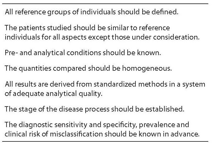
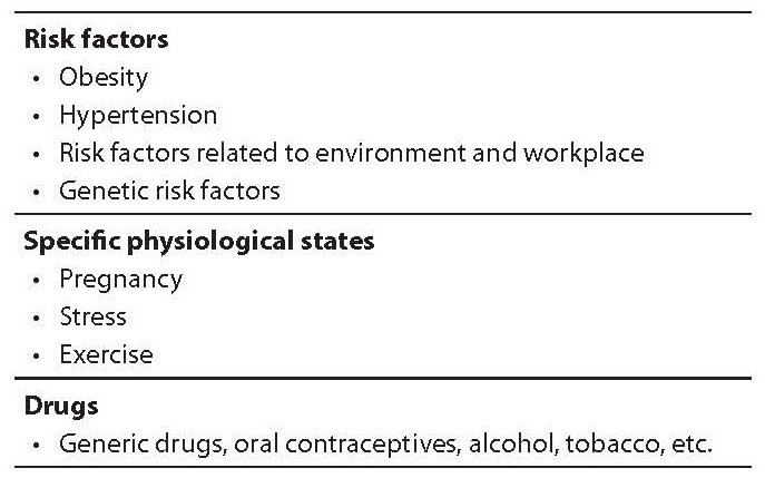
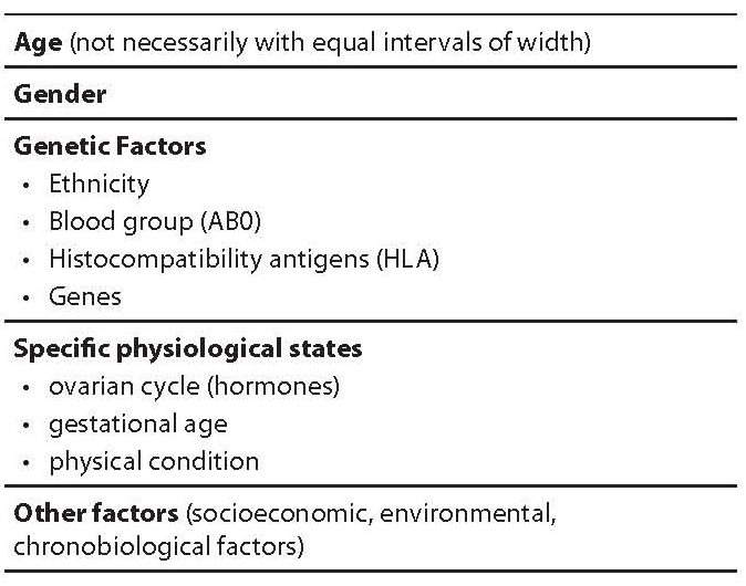
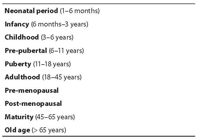
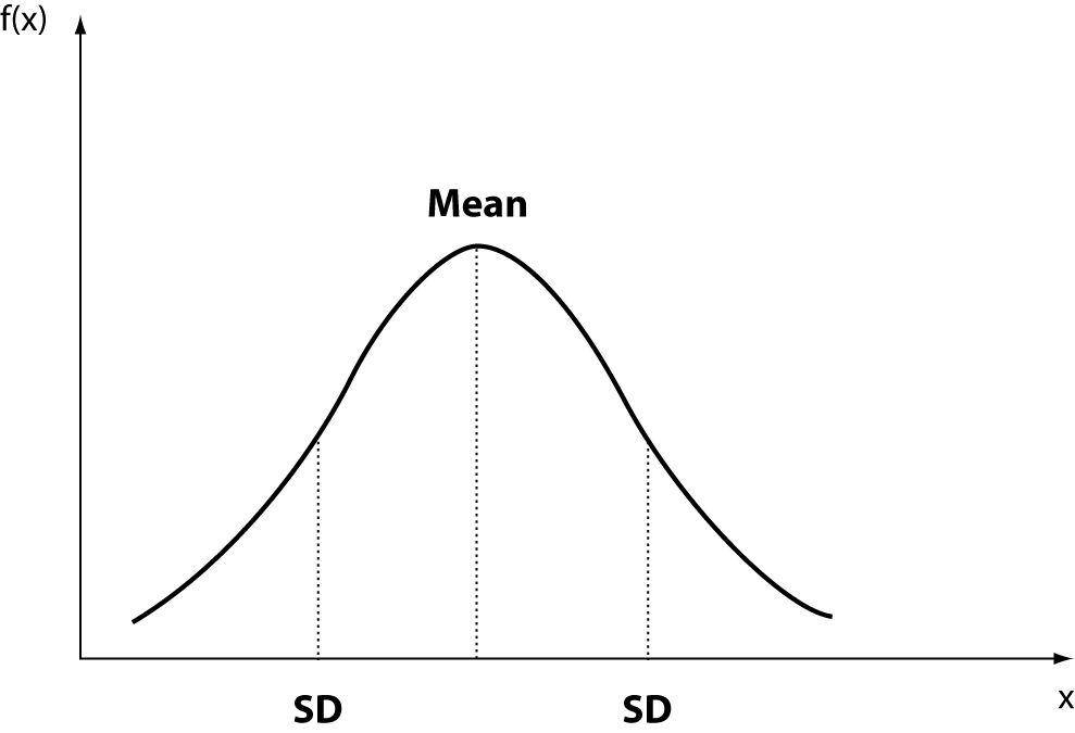


 Figure 5. Interval of reference: Gaussian curve.


 Figure 5. Interval of reference: Gaussian curve.